Google Contrails Forecasts
The Google Contrails API provides a global contrail forecast free of charge.
To access the Contrails API, use an API key from a GCP project with the Contrails API enabled. Then, set the GOOGLE_API_KEY environment variable to the API key or provide it in the constructor GoogleForecast(key='YOUR_API_KEY').
Alternatively, you can use any google-auth credentials, e.g. run gcloud auth application-default login to authenticate on your local machine.
[1]:
import cartopy.crs as ccrs
import matplotlib.pyplot as plt
import pandas as pd

from pycontrails.core.flight import Flight
from pycontrails.datalib.google_forecast import (
    ExpectedEffectiveEnergyForcing,
    GoogleForecast,
    Severity,
)
Download the Google Contrails forecast for 24h into the future
Request the Severity variable for a simple scale from 0 (no warming) to 4 (severe warming). Alternatively, request ExpectedEffectiveEnergyForcing for the expected, effective energy forcing in J/m. See the Google Contrails documentation for more details.
[2]:
gf = GoogleForecast(
    # The API provides hourly forecasts, up to +48h into the future.
    time=pd.Timestamp("2025-01-04T20:00:00Z"),
    variables=Severity,  # Also supports ExpectedEffectiveEnergyForcing.
    # key="YOUR_API_KEY",  # Optional if GOOGLE_API_KEY env var is set
)

met = gf.open_metdataset()
met
[2]:
MetDataset with data:
<xarray.Dataset> Size: 75MB
Dimensions:                  (longitude: 1441, latitude: 721, level: 18, time: 1)
Coordinates:
  * longitude                (longitude) float64 12kB -180.0 -179.8 ... 180.0
  * latitude                 (latitude) float64 6kB -90.0 -89.75 ... 89.75 90.0
  * level                    (level) float64 144B 154.7 162.4 ... 329.3 344.3
    flight_level             (level) int16 36B 440 430 420 410 ... 290 280 270
    air_pressure             (level) float32 72B 1.547e+04 ... 3.443e+04
    altitude                 (level) float32 72B 1.341e+04 ... 8.23e+03
  * time                     (time) datetime64[ns] 8B 2025-01-04T20:00:00
    forecast_reference_time  (time) datetime64[ns] 8B 2026-02-05T08:00:00
Data variables:
    contrails                (longitude, latitude, level, time) float32 75MB ...
Attributes:
    inference_pipeline_version:  contrails.forecast-pipeline_20260129.02_p0
    api_version:                 contrails.api-service_20260329.02_p0
    aircraft_class:              default
    provider:                    Google
    dataset:                     Contrails Forecast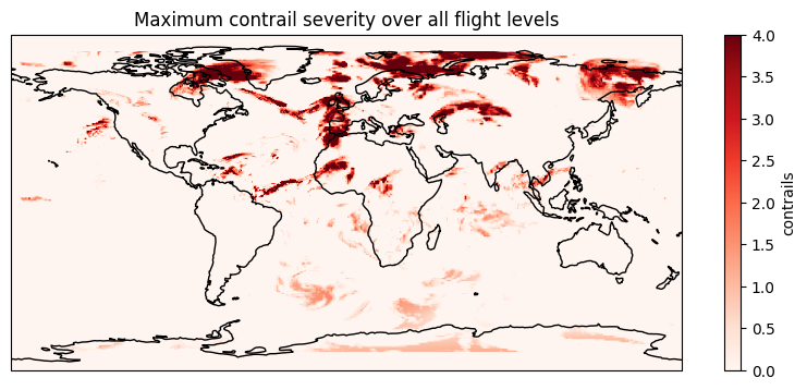
product: forecastPlot the forecasted contrail impact
[3]:
severity_da = met.data["contrails"].isel(time=0).max(dim="level")
p = severity_da.plot(
    x="longitude",
    y="latitude",
    cmap="Reds",
    subplot_kws=dict(projection=ccrs.PlateCarree(), transform=ccrs.PlateCarree()),
    figsize=(10, 4),
)
p.axes.coastlines()
plt.title("Maximum contrail severity over all flight levels");
Check the forecast for a specific flight trajectory
[4]:
# Load a sample flight.
df = pd.read_csv("../notebooks/data/flight-ap.csv", parse_dates=["time"])

# Hack: Because the sample flight is too far in the past, we "move" it to a more recent date.
# This is for demo purposes only and doesn't need to be done with any real flight plan!
df["time"] += pd.Timedelta(days=500)

fl = Flight(df)
fl
[4]:
Flight [4 keys x 130 length, 0 attributes]
| Attributes | |
|---|---|
| time | [2025-01-04 20:07:00, 2025-01-04 22:16:00] |
| longitude | [-97.01, -83.352] |
| latitude | [32.903, 42.229] |
| altitude | [190.5, 11582.4] |
| longitude | latitude | altitude | time | |
|---|---|---|---|---|
| 0 | -83.351920 | 42.228520 | 194.1576 | 2025-01-04 20:07:00 |
| 1 | -83.366890 | 42.208270 | 234.0864 | 2025-01-04 20:08:00 |
| 2 | -83.387894 | 42.181263 | 647.7000 | 2025-01-04 20:09:00 |
| 3 | -83.438850 | 42.129593 | 1089.6600 | 2025-01-04 20:10:00 |
| 4 | -83.499092 | 42.074844 | 1645.9200 | 2025-01-04 20:11:00 |
| ... | ... | ... | ... | ... |
| 125 | -97.008675 | 33.096130 | 1211.5800 | 2025-01-04 22:12:00 |
| 126 | -97.008942 | 33.043941 | 944.8800 | 2025-01-04 22:13:00 |
| 127 | -97.009109 | 32.992447 | 662.9400 | 2025-01-04 22:14:00 |
| 128 | -97.009560 | 32.946274 | 419.1000 | 2025-01-04 22:15:00 |
| 129 | -97.009727 | 32.903263 | 190.5000 | 2025-01-04 22:16:00 |
130 rows × 4 columns
Load the forecast for the entire flight duration
[7]:
# The forecast is provided hourly, so we round down the departure time, round up the arrival time, and load all hours inbetween.
global_mds = GoogleForecast(
    time=(fl.time_start.floor("h"), fl.time_end.ceil("h")),
    variables=ExpectedEffectiveEnergyForcing,
).open_metdataset()

global_mds
[7]:
MetDataset with data:
<xarray.Dataset> Size: 299MB
Dimensions:                            (longitude: 1441, latitude: 721,
                                        level: 18, time: 4)
Coordinates:
  * longitude                          (longitude) float64 12kB -180.0 ... 180.0
  * latitude                           (latitude) float64 6kB -90.0 ... 90.0
  * level                              (level) float64 144B 154.7 ... 344.3
    flight_level                       (level) int16 36B 440 430 420 ... 280 270
    air_pressure                       (level) float32 72B 1.547e+04 ... 3.44...
    altitude                           (level) float32 72B 1.341e+04 ... 8.23...
  * time                               (time) datetime64[ns] 32B 2025-01-04T2...
    forecast_reference_time            (time) datetime64[ns] 32B 2026-02-05T0...
Data variables:
    expected_effective_energy_forcing  (longitude, latitude, level, time) float32 299MB ...
Attributes:
    inference_pipeline_version:  contrails.forecast-pipeline_20260129.02_p0
    api_version:                 contrails.api-service_20260329.02_p0
    aircraft_class:              default
    provider:                    Google
    dataset:                     Contrails Forecast
product: forecastIntersect the forecast with the flight trajectory
[8]:
fl = fl.resample_and_fill()
fl["eeef_per_m"] = fl.intersect_met(
    global_mds["expected_effective_energy_forcing"],
    method="linear",
    fill_value=0.0,
)
fl.dataframe[["eeef_per_m"]].describe()
[8]:
| eeef_per_m | |
|---|---|
| count | 1.300000e+02 |
| mean | 4.886437e+05 |
| std | 8.505285e+05 |
| min | 0.000000e+00 |
| 25% | 0.000000e+00 |
| 50% | 5.245293e+04 |
| 75% | 5.177957e+05 |
| max | 4.006021e+06 |
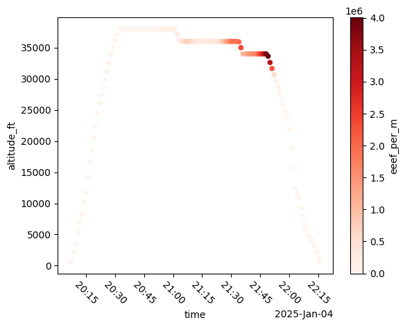
Plot the expected effective energy forcing for the flight’s vertical profile
[9]:
fl.plot_profile(kind="scatter", c="eeef_per_m", cmap="Reds", rot=-45);
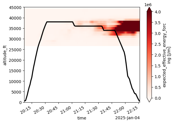
Draw a curtain plot of the contrail forecast behind the flight’s vertical profile
[10]:
fig, ax = plt.subplots()

eeef_curtain = fl.intersect_met_cross_section(
    global_mds["expected_effective_energy_forcing"], dim="level"
)
eeef_curtain.plot.pcolormesh(
    x="time",
    y="altitude_ft",
    ax=ax,
    cmap="Reds",
    vmin=0,
    vmax=4e6,  # Hardcode same color scale as above.
    ylim=(0, 45000),
)

# Overlay the `flight.plot_profile` natively onto the same axis. Requires x_compat to use the same x-axis.
fl.plot_profile(ax=ax, color="black", linewidth=2.5, label="Flight Overlaid", x_compat=True);
/usr/local/google/home/maxvo/Projects/pycontrails/venv/lib/python3.13/site-packages/pandas/plotting/_matplotlib/core.py:981: UserWarning: This axis already has a converter set and is updating to a potentially incompatible converter
  return ax.plot(*args, **kwds)