APCEMM

Pycontrails interface for the MIT Aircraft Plume Chemistry Emission and Microphysics Model (APCEMM).

This interface runs APCEMM simulations initialized at waypoints in a pycontrails Flight.

References

Fritz, Thibaud M., Sebatian D. Eastham, Raymond L. Speth, and Steven R.H. Barret. “The role of plume-scale processes in long-term impacts of aircraft emissions.” Atmospheric Chemistry and Physics 20, no. 9 (May 13, 2020): 5697–727. https://doi.org/10.5194/acp-20-5697-2020.

import os

import cartopy.crs as ccrs
import matplotlib.pyplot as plt
import numpy as np
import pandas as pd
import xarray as xr
from matplotlib import colors

from pycontrails import Flight, MetVariable
from pycontrails.core.met_var import Geopotential
from pycontrails.datalib.ecmwf import ERA5ARCO
from pycontrails.models.apcemm.apcemm import APCEMM
from pycontrails.models.humidity_scaling import HistogramMatching
from pycontrails.models.issr import ISSR
from pycontrails.models.ps_model import PSFlight
from pycontrails.physics import thermo, units

plt.rcParams["figure.figsize"] = (10, 6)

Download meteorology data

This demo uses model-level ERA5 data from the ARCO ERA5 dataset for met data.

Note this will download ~3 GB of meteorology data to your computer

time_bounds = ("2019-01-01 00:00:00", "2019-01-01 04:00:00")

variables = (v if isinstance(v, MetVariable) else Geopotential for v in APCEMM.met_variables)
era5ml = ERA5ARCO(time=time_bounds, variables=APCEMM.met_variables)

met = era5ml.open_metdataset(wrap_longitude=True)

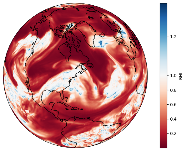
Plot RHI at FL350

fl350 = met.data.sel(level=units.ft_to_pl(35_000), method="nearest")

rhi = thermo.rhi(fl350["specific_humidity"], fl350["air_temperature"], fl350["air_pressure"])

ax = plt.subplot(
    111, projection=ccrs.NearsidePerspective(central_longitude=-71.1, central_latitude=42.3)
)
ax.coastlines()
im = ax.pcolormesh(
    rhi["longitude"],
    rhi["latitude"],
    rhi.isel(time=0).T,
    shading="nearest",
    transform=ccrs.PlateCarree(),
    cmap="RdBu",
    norm=colors.TwoSlopeNorm(vcenter=1.0),
)
plt.colorbar(im, label="RHI");

Load Flight Data

A Flight can be loaded from CSV or Parquet files or created from a pandas DataFrame. Here, we create a synthetic flight between Chicago and Boston at 35,000 ft.

flight_attrs = {
    "flight_id": "test",
    "aircraft_type": "B738",
}

df = pd.DataFrame()
df["longitude"] = np.array([-87.6298, -71.0589])
df["latitude"] = np.array([41.8781, 42.3601])
df["altitude_ft"] = np.array([35_000.0, 35_000.0])
df["time"] = np.array([np.datetime64("2019-01-01 01:00"), np.datetime64("2019-01-01 02:15")])

flight = Flight(df, attrs=flight_attrs).resample_and_fill("1min")

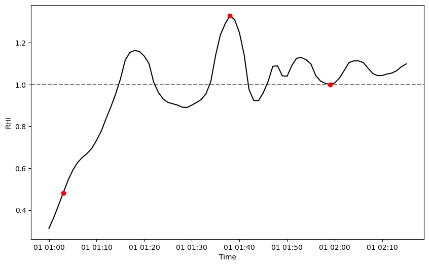
Select waypoints for evaluation with APCEMM

We use the ISSR model to select waypoints with varying RHi.

# model ISSR
model = ISSR(met, humidity_scaling=HistogramMatching(level_type="model"))
result = model.eval(flight, copy_source=True)

# select a few waypoints
waypoints = [3, 38, 59]

# plot select waypoints on ISSR results
plt.plot(result["time"], result["rhi"], "k-")
for waypoint in waypoints:
    plt.plot(result["time"][waypoint], result["rhi"][waypoint], "ro")
plt.xlabel("Time")
plt.ylabel("RHI")
plt.gca().axhline(y=1, color="gray", ls="--", zorder=-1);

Run APCEMM on selected flight segments

The pycontrails interface assumes that APCEMM is installed at $HOME/APCEMM when generating input YAML files, but a different root directory can be specified using the apcemm_root parameter.

The max_age parameter should be longer than 1 hour to simulate the full lifecycle of persistent contrails. We use a small value to keep the simulation runtime relatively short.

apcemm_root = f"{os.getenv('HOME')}/Files/Code/contrails/APCEMM"

model = APCEMM(
    apcemm_path=f"{apcemm_root}/build/APCEMM",
    apcemm_root=apcemm_root,
    met=met,
    max_age=np.timedelta64(1, "h"),
    aircraft_performance=PSFlight(),
    humidity_scaling=HistogramMatching(level_type="model"),
)

Setting n_jobs = 3 runs simulations for all three waypoints in parallel.

result = model.eval(flight, waypoints=waypoints, n_jobs=3)

Print status of APCEMM simulations

for waypoint in waypoints:
    print(f"Waypoint {waypoint}: {result.dataframe.iloc[waypoint]['status']}")

Waypoint 3: NoWaterSaturation
Waypoint 38: Incomplete
Waypoint 59: NoPersistence

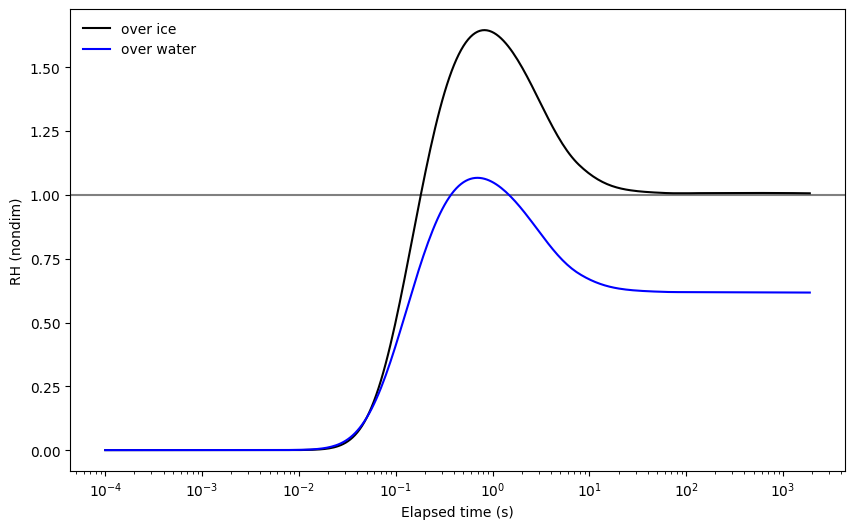
Plot output from the early plume model

df = model.vortex
df = df[df["waypoint"] == 38].sort_values("time")

elapsed_time = (df["time"] - flight.dataframe.iloc[38]["time"]).dt.total_seconds()
plt.plot(elapsed_time, df["RH_i [-]"], "k-", label="over ice")
plt.plot(elapsed_time, df["RH_w [-]"], "b-", label="over water")
plt.gca().set_xscale("log")
plt.xlabel("Elapsed time (s)")
plt.ylabel("RH (nondim)")
plt.legend(loc="upper left", frameon=False)
plt.gca().axhline(y=1, color="gray", zorder=-1)

<matplotlib.lines.Line2D at 0x7492e4728e90>

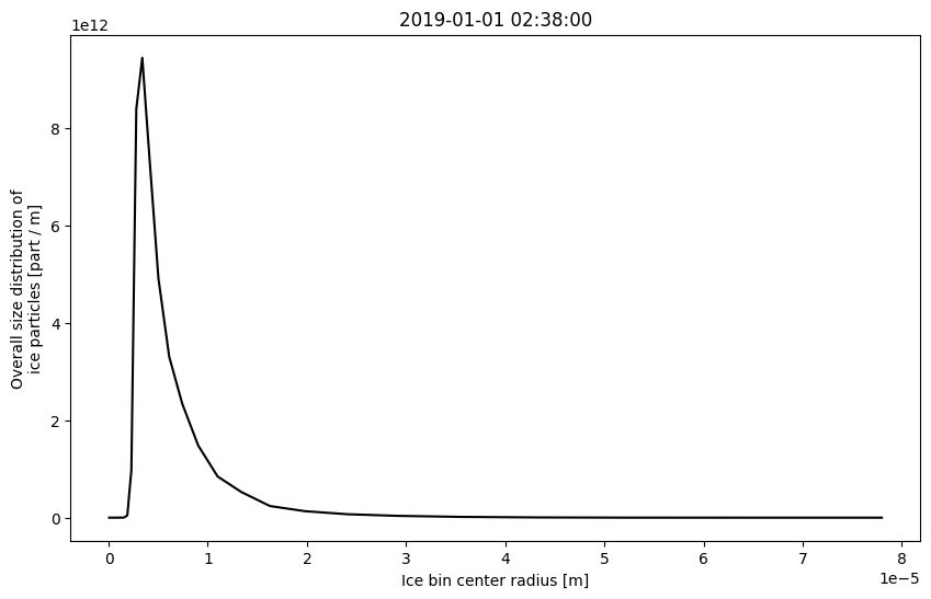
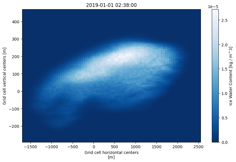
Plot netCDF output from the finite-volume contrail cross-section model

df = model.contrail
df = df[df["waypoint"] == 38]

ds = xr.open_dataset(df.iloc[-1].path, decode_times=False)

ds["IWC"].plot(cmap="Blues_r")
plt.title(df.iloc[-1]["time"]);

ds["Overall size distribution"].plot(color="k")
plt.title(df.iloc[-1]["time"]);