Run CoCiP with FDR or QAR data¶

References¶

Schumann, U. “A Contrail Cirrus Prediction Model.” Geoscientific Model Development 5, no. 3 (May 3, 2012): 543–80. https://doi.org/10.5194/gmd-5-543-2012.
EASA: ICAO Aircraft Engine Emissions Databank (07/2021), 2021.
ICAO: Annex 16: Environmental Protection - Volume II - Aircraft Engine Emissions: https://store.icao.int/en/annex-16-environmental-protection-volume-ii-aircraft-engine-emissions, 2008. Last access: 18 August 2022.

[1]:

import numpy as np
import xarray as xr
import pandas as pd
from matplotlib import pyplot as plt
import scipy

from pycontrails import Flight
from pycontrails.datalib.ecmwf import ERA5
from pycontrails.models.cocip import Cocip
from pycontrails.models.humidity_scaling import HistogramMatching
from pycontrails.models.ps_model import PSFlight
from pycontrails.models.emissions import Emissions

Download met data¶

[2]:

time_bounds = ("2022-03-01 00:00:00", "2022-03-01 23:00:00")
pressure_levels = (300, 250, 200)  # 30,000 ft to 38,000 ft

era5pl = ERA5(
    time=time_bounds,
    variables=Cocip.met_variables + Cocip.optional_met_variables,
    pressure_levels=pressure_levels,
)
era5sl = ERA5(time=time_bounds, variables=Cocip.rad_variables)

# download data from ERA5 (or open from cache)
met = era5pl.open_metdataset()
rad = era5sl.open_metdataset()

Read in data and resample¶

In this example, the sample data provides TAS, aircraft mass, and fuel flow per engine. Any values provided as input to the CoCiP model will not be overwritten when CoCiP is run, and so we should make sure we are saving the most accurate portions of the FDR data. Typically, thurst values provided by FDRs are noisy and innaccurate and so it is recommended to drop the thrust value if provided and recompute thrust through an aircraft performance model (below).

In this case, fuel flow is provided per engine, and so total fuel flow must be computed by summing the two values together.

Here we are also resampling the FDR data to a one minute sampling period, which is recommended when running CoCiP. Note that the resample_and_fill function will interpolate time, position, and altitude, but for the remaining columns, it will simply choose the nearsest value. There are much more accurate ways to resample fuel flow data, but this should generally be sufficient to estimate contrail impacts.

[3]:

attrs = {
    "flight_id": "test",
    "aircraft_type": "B77W",
    "engine_uid": "01P21GE217",  # 01P21GE217 -> GE90-115B
    # "n_engine":2 # This shouldn't be needed?
}

df = pd.read_csv("data/flight-fdr.csv")
df["fuel_flow"] = df["fuel_flow_1"] + df["fuel_flow_2"]  # Checked
fl = Flight(df, attrs=attrs)

fl = fl.resample_and_fill(freq="60s", drop=False)
fl

[3]:

Flight [10 keys x 136 length, 4 attributes]

Attributes
time	[2022-03-01 00:15:00, 2022-03-01 02:30:00]
longitude	[-39.926, -25.0]
latitude	[34.0, 39.97]
altitude	[10900.0, 10900.0]
flight_id	test
aircraft_type	B77W
engine_uid	01P21GE217
crs	EPSG:4326

	longitude	latitude	altitude	flight_id	true_airspeed	aircraft_mass	fuel_flow_1	fuel_flow_2	fuel_flow	time
0	-25.000000	34.000000	10900.0	test	215.628175	237650.498951	0.786975	0.786975	1.573950	2022-03-01 00:15:00
1	-25.111111	34.044444	10900.0	test	215.906118	237556.061693	0.786984	0.786984	1.573968	2022-03-01 00:16:00
2	-25.220370	34.088148	10900.0	test	216.176652	237463.196123	0.787013	0.787013	1.574027	2022-03-01 00:17:00
3	-25.331481	34.132593	10900.0	test	216.433880	237368.802459	0.786496	0.786496	1.572992	2022-03-01 00:18:00
4	-25.442593	34.177037	10900.0	test	216.684851	237274.417192	0.786600	0.786600	1.573200	2022-03-01 00:19:00
...	...	...	...	...	...	...	...	...	...	...
131	-39.483333	39.793333	10900.0	test	230.120409	225427.222884	0.775681	0.775681	1.551362	2022-03-01 02:26:00
132	-39.594444	39.837778	10900.0	test	230.055073	225334.320532	0.773240	0.773240	1.546479	2022-03-01 02:27:00
133	-39.703704	39.881481	10900.0	test	229.945472	225243.173069	0.771585	0.771585	1.543171	2022-03-01 02:28:00
134	-39.814815	39.925926	10900.0	test	229.772775	225150.752744	0.768882	0.768882	1.537763	2022-03-01 02:29:00
135	-39.925926	39.970370	10900.0	test	229.550583	225058.592246	0.767088	0.767088	1.534177	2022-03-01 02:30:00

136 rows × 10 columns

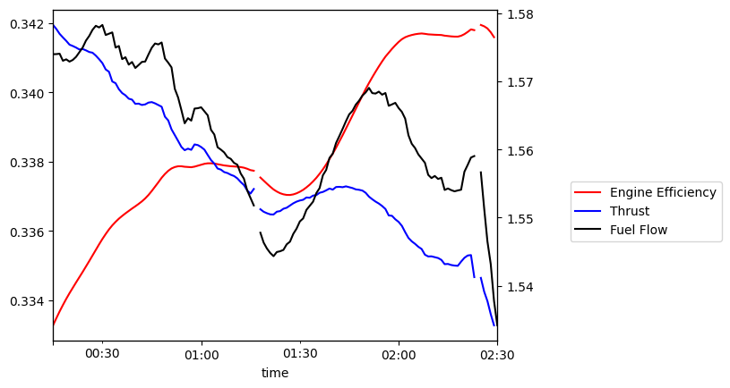
(Optional) Run Aircraft Performance Model¶

The CoCiP module will automatically run an aircraft performance model to compute any missing values needed. In this case, we still need to compute engine efficiency and estimated thrust force. For completeness, we show how this can be computed directly from the an aircraft performance model.

[4]:

perf = PSFlight(met=met)
fp = perf.eval(fl)

[5]:

fig, ax = plt.subplots()
ax2 = ax.twinx()
ax3 = ax2.twinx()
ax2.set_yticks([])
fp.dataframe.plot(ax=ax, x="time", y="engine_efficiency", style="r", legend=False)
fp.dataframe.plot(ax=ax2, x="time", y="thrust", style="b", legend=False)
fp.dataframe.plot(ax=ax3, x="time", y="fuel_flow", style="k", legend=False)
_ = ax3.legend(
    [ax.get_lines()[0], ax2.get_lines()[0], ax3.get_lines()[0]],
    ["Engine Efficiency", "Thrust", "Fuel Flow"],
    bbox_to_anchor=(1.15, 0.5),
)

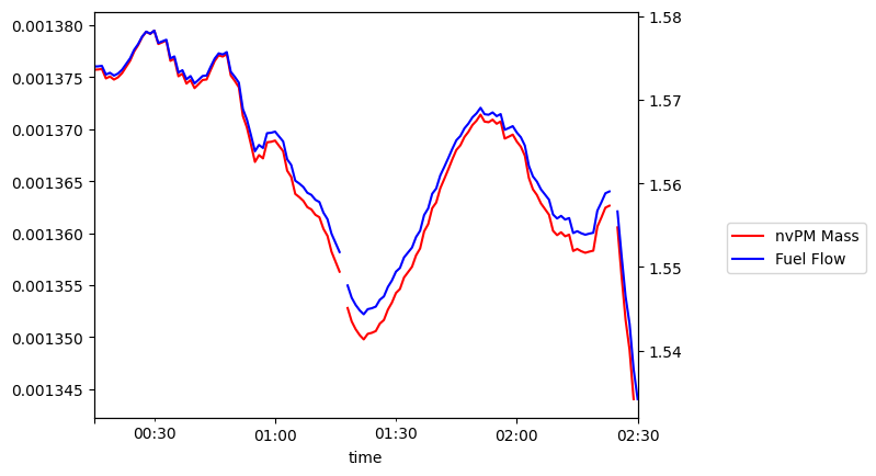
../_images/notebooks_run-cocip-with-fdr_10_0.png

Compute Aircraft Emissions¶

Given fuel flow data, met data, aircraft, and engine type, we have sufficient information to run the emissions module and compute nvPM estimates needed as input for CoCiP. We have not specified engine type, so in the case, the default engine type will be assumed, which for the B77W is the GE-90 115B. To specific a different engine type, add the key engine_uid to the attrs dict when creating the Flight object.

Note that the emissions module estimates the aircraft thrust setting by comparing the fuel flow to the maximum fuel flow. This is the perferred way to estimate emissions using the ICAO emissions inventory and is the default behavior of the emissions module even when aircraft thrust is provided in the input.

[6]:

emissions = Emissions(met=met, humidity_scaling=HistogramMatching())
fl = emissions.eval(fl)
fl

[6]:

Flight [31 keys x 136 length, 17 attributes]

Attributes
time	[2022-03-01 00:15:00, 2022-03-01 02:30:00]
longitude	[-39.926, -25.0]
latitude	[34.0, 39.97]
altitude	[10900.0, 10900.0]
flight_id	test
aircraft_type	B77W
engine_uid	01P21GE217
crs	EPSG:4326
n_engine	2
gaseous_data_source	FFM2
nvpm_data_source	ICAO EDB
total_co2	39390.76441156896
total_h2o	15337.3346711712
total_so2	14.963253337727998
total_sulphates	0.30537251709648977
total_oc	0.2493875556288
total_nox	192.979281298076
total_co	2.915210297723201
total_hc	0.6230983842461807
total_nvpm_mass	0.18164446517898938
total_nvpm_number	3.54753797881968e+18

	longitude	latitude	altitude	flight_id	true_airspeed	aircraft_mass	fuel_flow_1	fuel_flow_2	fuel_flow	time	...	co2	h2o	so2	sulphates	oc	nox	co	hc	nvpm_mass	nvpm_number
0	-25.000000	34.000000	10900.0	test	215.628175	237650.498951	0.786975	0.786975	1.573950	2022-03-01 00:15:00	...	298.326415	116.157483	0.113324	0.002313	0.001889	1.450262	0.021463	0.004587	0.001376	2.686732e+16
1	-25.111111	34.044444	10900.0	test	215.906118	237556.061693	0.786984	0.786984	1.573968	2022-03-01 00:16:00	...	298.329927	116.158851	0.113326	0.002313	0.001889	1.450494	0.021460	0.004587	0.001376	2.686764e+16
2	-25.220370	34.088148	10900.0	test	216.176652	237463.196123	0.787013	0.787013	1.574027	2022-03-01 00:17:00	...	298.340990	116.163158	0.113330	0.002313	0.001889	1.450803	0.021459	0.004587	0.001376	2.686863e+16
3	-25.331481	34.132593	10900.0	test	216.433880	237368.802459	0.786496	0.786496	1.572992	2022-03-01 00:18:00	...	298.144830	116.086781	0.113255	0.002311	0.001888	1.449472	0.021447	0.004584	0.001375	2.685097e+16
4	-25.442593	34.177037	10900.0	test	216.684851	237274.417192	0.786600	0.786600	1.573200	2022-03-01 00:19:00	...	298.184382	116.102181	0.113270	0.002312	0.001888	1.450112	0.021455	0.004586	0.001375	2.685453e+16
...	...	...	...	...	...	...	...	...	...	...	...	...	...	...	...	...	...	...	...	...	...
131	-39.483333	39.793333	10900.0	test	230.120409	225427.222884	0.775681	0.775681	1.551362	2022-03-01 02:26:00	...	294.045243	114.490550	0.111698	0.002280	0.001862	1.444279	0.022017	0.004706	0.001356	2.648176e+16
132	-39.594444	39.837778	10900.0	test	230.055073	225334.320532	0.773240	0.773240	1.546479	2022-03-01 02:27:00	...	293.119693	114.130175	0.111347	0.002272	0.001856	1.436100	0.021918	0.004685	0.001352	2.639840e+16
133	-39.703704	39.881481	10900.0	test	229.945472	225243.173069	0.771585	0.771585	1.543171	2022-03-01 02:28:00	...	292.492624	113.886017	0.111108	0.002268	0.001852	1.430317	0.021840	0.004668	0.001349	2.634193e+16
134	-39.814815	39.925926	10900.0	test	229.772775	225150.752744	0.768882	0.768882	1.537763	2022-03-01 02:29:00	...	291.467679	113.486941	0.110719	0.002260	0.001845	1.421186	0.021731	0.004645	0.001344	2.624962e+16
135	-39.925926	39.970370	10900.0	test	229.550583	225058.592246	0.767088	0.767088	1.534177	2022-03-01 02:30:00	...	NaN	NaN	NaN	NaN	NaN	NaN	NaN	NaN	NaN	NaN

136 rows × 31 columns

[7]:

fig, ax = plt.subplots()
ax2 = ax.twinx()
fl.dataframe.plot(ax=ax, x="time", y="nvpm_mass", style="r", legend=False)
fl.dataframe.plot(ax=ax2, x="time", y="fuel_flow", style="b", legend=False)
ax2.legend(
    [
        ax.get_lines()[0],
        ax2.get_lines()[0],
    ],
    ["nvPM Mass", "Fuel Flow"],
    bbox_to_anchor=(1.15, 0.5),
)

[7]:

<matplotlib.legend.Legend at 0x176d15010>

../_images/notebooks_run-cocip-with-fdr_13_1.png

Run CoCiP over the flight¶

In order to predict contrail impact, we still need an estimate of engine efficiency, which is needed to determine if the Schmidt-Appleman Criteria is satisfied. If we provide the CoCiP module with an aircraft performance model, in this case the Poll-Schumann model, then this value will be estimated for us.

In the code below, the CoCiP module will run the Poll-Schmann model over the flight using the provided aircraft mass in order to estimate the thrust force required for the plane to fly the specified trajectory. This value will then be used along with the provided fuel flow data to estimate engine efficiency. Fuel flow and emissions numbers will not be recomputed here, and the warning from aircraft_performance.py can be ignored — three iterations of the performance model are only needed to estimate aircraft mass, which in this case is taken from the FDR data.

[8]:

cocip = Cocip(
    met=met, rad=rad, aircraft_performance=PSFlight(), humidity_scaling=HistogramMatching()
)
fl = cocip.eval(fl)
fl

[8]:

Flight [67 keys x 136 length, 25 attributes]

Attributes
time	[2022-03-01 00:15:00, 2022-03-01 02:30:00]
longitude	[-39.926, -25.0]
latitude	[34.0, 39.97]
altitude	[10900.0, 10900.0]
flight_id	test
aircraft_type	B77W
engine_uid	01P21GE217
crs	EPSG:4326
n_engine	2
gaseous_data_source	FFM2
nvpm_data_source	ICAO EDB
total_co2	39390.76441156896
total_h2o	15337.3346711712
total_so2	14.963253337727998
total_sulphates	0.30537251709648977
total_oc	0.2493875556288
total_nox	192.979281298076
total_co	2.915210297723201
total_hc	0.6230983842461807
total_nvpm_mass	0.18164446517898938
total_nvpm_number	3.54753797881968e+18
aircraft_performance_model	PSFlight
wingspan	64.8
max_mach	0.89
max_altitude	13136.880000000001
total_fuel_burn	12469.37778144
humidity_scaling_name	histogram_matching
humidity_scaling_formula	era5_quantiles -> iagos_quantiles
pycontrails_version	0.49.3.dev50

	waypoint	longitude	latitude	altitude	flight_id	true_airspeed	aircraft_mass	fuel_flow_1	fuel_flow_2	fuel_flow	...	n_ice_per_m_1	ef	contrail_age	sdr_mean	rsr_mean	olr_mean	rf_sw_mean	rf_lw_mean	rf_net_mean	cocip
0	0	-25.000000	34.000000	10900.0	test	215.628175	237650.498951	0.786975	0.786975	1.573950	...	NaN	0.0	0 days	NaN	NaN	NaN	NaN	NaN	NaN	0.0
1	1	-25.111111	34.044444	10900.0	test	215.906118	237556.061693	0.786984	0.786984	1.573968	...	NaN	0.0	0 days	NaN	NaN	NaN	NaN	NaN	NaN	0.0
2	2	-25.220370	34.088148	10900.0	test	216.176652	237463.196123	0.787013	0.787013	1.574027	...	NaN	0.0	0 days	NaN	NaN	NaN	NaN	NaN	NaN	0.0
3	3	-25.331481	34.132593	10900.0	test	216.433880	237368.802459	0.786496	0.786496	1.572992	...	NaN	0.0	0 days	NaN	NaN	NaN	NaN	NaN	NaN	0.0
4	4	-25.442593	34.177037	10900.0	test	216.684851	237274.417192	0.786600	0.786600	1.573200	...	2.453534e+10	0.0	0 days	NaN	NaN	NaN	NaN	NaN	NaN	0.0
...	...	...	...	...	...	...	...	...	...	...	...	...	...	...	...	...	...	...	...	...	...
131	131	-39.483333	39.793333	10900.0	test	230.120409	225427.222884	0.775681	0.775681	1.551362	...	NaN	0.0	0 days	NaN	NaN	NaN	NaN	NaN	NaN	0.0
132	132	-39.594444	39.837778	10900.0	test	230.055073	225334.320532	0.773240	0.773240	1.546479	...	NaN	0.0	0 days	NaN	NaN	NaN	NaN	NaN	NaN	0.0
133	133	-39.703704	39.881481	10900.0	test	229.945472	225243.173069	0.771585	0.771585	1.543171	...	NaN	0.0	0 days	NaN	NaN	NaN	NaN	NaN	NaN	0.0
134	134	-39.814815	39.925926	10900.0	test	229.772775	225150.752744	0.768882	0.768882	1.537763	...	NaN	0.0	0 days	NaN	NaN	NaN	NaN	NaN	NaN	0.0
135	135	-39.925926	39.970370	10900.0	test	229.550583	225058.592246	0.767088	0.767088	1.534177	...	NaN	0.0	0 days	NaN	NaN	NaN	NaN	NaN	NaN	0.0

136 rows × 67 columns

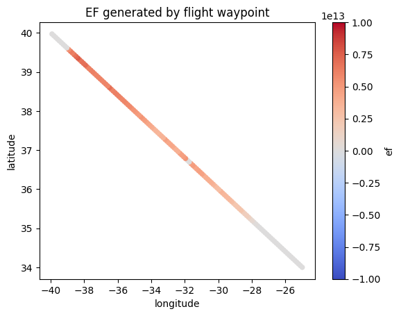
Visualize Contrail Impact¶

First, we plot cumulative EF by flight waypoint (one minute sample period)

[9]:

fl.dataframe.plot.scatter(
    x="longitude",
    y="latitude",
    c="ef",
    cmap="coolwarm",
    vmin=-1e13,
    vmax=1e13,
    title="EF generated by flight waypoint",
);

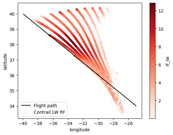
../_images/notebooks_run-cocip-with-fdr_17_0.png

Next, we plot the evolution of the contrail as it advects along each flight segment

[10]:

ax = plt.axes()

cocip.source.dataframe.plot(
    "longitude",
    "latitude",
    color="k",
    ax=ax,
    label="Flight path",
)
cocip.contrail.plot.scatter(
    "longitude",
    "latitude",
    c="rf_lw",
    cmap="Reds",
    ax=ax,
    label="Contrail LW RF",  # Contrail age?
)
ax.legend();

../_images/notebooks_run-cocip-with-fdr_19_0.png