Working with Model Level Met¶

Meteorology providers may choose to compute their data on different vertical levels. For example, the ECMWF IFS product is computed on 137 model levels. The pressure of a given model level is not constant, but varies with time and horizontal position. The pressure at a given point can be computed following ECMWF guidelines. This notebook uses the metview library to convert from ECMWF model levels to pressure levels.

The metview package can be difficult to install. Installation with conda may be the easiest way to get started. This notebook assumes a working installation of metview.

[1]:

import os

import cdsapi
import matplotlib.pyplot as plt
import metview as mv
import numpy as np
import pandas as pd
import xarray as xr

from pycontrails import Fleet, Flight, MetDataset
from pycontrails.datalib.ecmwf import PRESSURE_LEVEL_VARIABLES, SURFACE_VARIABLES
from pycontrails.models.cocip import Cocip
from pycontrails.models.humidity_scaling import HistogramMatching
from pycontrails.models.ps_model import PSFlight

Define CDS model level request¶

We make three requests to the CDS API.

ml_request is a request for the model levels meteorology data
lnsp_request is a request for the surface pressure data needed for interpolating from model levels to pressure levels
sl_request is a request for the single level top of atmosphere radiation data needed for CoCiP

[2]:

date = "2024-01-15"
time = list(range(18))
grid = "1/1"

ml_variables = ["t", "q", "u", "v", "w", "ciwc"]
sl_variables = ["tsr", "ttr"]

ml_request = {
    "levtype": "ml",
    "levellist": "70/to/90/by/1",
    "param": ml_variables,
    "date": date,
    "time": time,
    "grid": grid,
}

lnsp_request = {
    "levtype": "ml",
    "levelist": "1",
    "param": "lnsp",
    "date": date,
    "time": time,
    "grid": grid,
}

sl_request = {
    "levtype": "sfc",
    "product_type": "reanalysis",
    "param": sl_variables,
    "date": date,
    "time": time,
    "grid": grid,
    "format": "netcdf",
}

Make the request¶

Download the data if it is not already sitting on disk. Depending on the load on the Copernicus server, we may get queued here for a while.

[3]:

client = cdsapi.Client()

target = "ml.grib"
if not os.path.isfile(target):
    client.retrieve("reanalysis-era5-complete", ml_request, target)

target = "lnsp.grib"
if not os.path.isfile(target):
    client.retrieve("reanalysis-era5-complete", lnsp_request, target)

target = "sl.nc"
if not os.path.isfile(target):
    client.retrieve("reanalysis-era5-single-levels", sl_request, target)

Target pressure levels¶

In order to use the metview library to convert from model levels to pressure levels, we must specify target pressure levels for the re-interpolation.

Assuming a constant surface pressure of 1013.25 hPa, the table below shows that ECMWF model levels occur roughly every 10 hPa at altitudes for which contrails form. This informs how we set our target pressure levels: We define our target pressure levels ranging from 170 hPa to 390 hPa, spaced every 10 hPa. A finer spacing than this may be redundant (pycontrails models perform linear interpolation between pressure levels), and a coarser spacing would result in loss of information.

[4]:

url = "https://confluence.ecmwf.int/display/UDOC/L137+model+level+definitions"
df = pd.read_html(url, na_values="-", index_col="n")[0].rename_axis("hybrid")
df.loc[70:90]  # model levels 70 - 90 agree with our ml_request

[4]:

	a [Pa]	b	ph [hPa]	pf [hPa]	Geopotential Altitude [m]	Geometric Altitude [m]	Temperature [K]	Density [kg/m^3]
hybrid
70	15508.256836	0.011806	167.0450	163.0927	13077.79	13104.70	216.65	0.262244
71	16026.115234	0.014816	175.2731	171.1591	12771.64	12797.30	216.65	0.275215
72	16527.322266	0.018318	183.8344	179.5537	12467.99	12492.44	216.65	0.288713
73	17008.789063	0.022355	192.7389	188.2867	12166.81	12190.10	216.65	0.302755
74	17467.613281	0.026964	201.9969	197.3679	11868.08	11890.24	216.65	0.317357
75	17901.621094	0.032176	211.6186	206.8078	11571.79	11592.86	216.65	0.332536
76	18308.433594	0.038026	221.6146	216.6166	11277.92	11297.93	216.65	0.348308
77	18685.718750	0.044548	231.9954	226.8050	10986.70	11005.69	216.74	0.364545
78	19031.289063	0.051773	242.7719	237.3837	10696.22	10714.22	218.62	0.378253
79	19343.511719	0.059728	253.9549	248.3634	10405.61	10422.64	220.51	0.392358
80	19620.042969	0.068448	265.5556	259.7553	10114.89	10130.98	222.40	0.406868
81	19859.390625	0.077958	277.5852	271.5704	9824.08	9839.26	224.29	0.421790
82	20059.931641	0.088286	290.0548	283.8200	9533.20	9547.49	226.18	0.437130
83	20219.664063	0.099462	302.9762	296.5155	9242.26	9255.70	228.08	0.452897
84	20337.863281	0.111505	316.3607	309.6684	8951.30	8963.90	229.97	0.469097
85	20412.308594	0.124448	330.2202	323.2904	8660.32	8672.11	231.86	0.485737
86	20442.078125	0.138313	344.5663	337.3932	8369.35	8380.36	233.75	0.502825
87	20425.718750	0.153125	359.4111	351.9887	8078.41	8088.67	235.64	0.520367
88	20361.816406	0.168910	374.7666	367.0889	7787.51	7797.04	237.53	0.538370
89	20249.511719	0.185689	390.6450	382.7058	7496.68	7505.51	239.42	0.556842
90	20087.085938	0.203491	407.0583	398.8516	7205.93	7214.09	241.31	0.575790

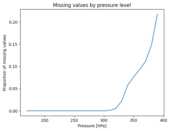
Missing values¶

Converting from model levels to pressure levels will result in some missing values. These are plotted below.

Points at which the surface pressure is significantly lower than the 1013.25 hPa reference surface pressure will result in missing values at the lowest-altitude target pressure levels. Additional model levels can be downloaded to decrease the number of missing values. Missing values do not occur at higher-altitude target pressure levels.

[7]:

da = met.data["air_temperature"]
da.isnull().groupby("level").mean(...).plot()
plt.ylabel("Proportion of missing values")
plt.title("Missing values by pressure level");

../_images/notebooks_model-levels_12_0.png

[8]:

# There are no missing values above 310 hPa
tmp = da.isnull().isel(time=0).sel(level=slice(310, None))
tmp.plot(x="longitude", y="latitude", add_colorbar=False, col="level", col_wrap=3)
plt.gcf().suptitle("Position of missing values by pressure level", y=1.02);

../_images/notebooks_model-levels_13_0.png

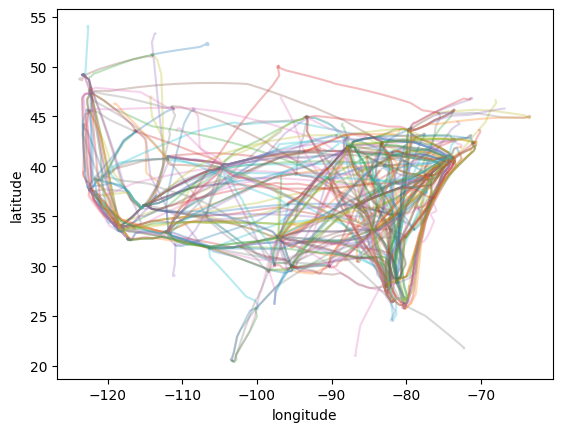
Download ADS-B¶

For flight trajectories, we use a sample from Contrails API. We artificially shift the times of the flight trajectories to overlap the times of the ERA5 data.

[10]:

df = pd.read_csv("https://apidocs.contrails.org/_static/fleet_sample.csv", parse_dates=["time"])
df["time"] = df["time"].dt.tz_convert(None)
df = df.rename(columns={"altitude": "altitude_ft"})

# Shift time to the date of interest
df["time"] = df["time"] + (pd.Timestamp(date) - df["time"].min())

# Convert to a pycontrails Fleet instance, keeping only aircraft type covered by the PS model
ps_flight = PSFlight()
flights = []
for flight_id, group in df.groupby("flight_id"):
    aircraft_type = group["aircraft_type"].iloc[0]
    if not ps_flight.check_aircraft_type_availability(aircraft_type, raise_error=False):
        continue

    engine_uid = group["engine_uid"].iloc[0]
    group = group.drop(columns=["aircraft_type", "engine_uid", "flight_id"])
    flight = Flight(group, aircraft_type=aircraft_type, engine_uid=engine_uid, flight_id=flight_id)
    flights.append(flight)

fleet = Fleet.from_seq(flights)

[11]:

ax = plt.subplot()
for flight in flights:
    flight.plot(ax=ax, alpha=0.3)

../_images/notebooks_model-levels_18_0.png

Run CoCiP¶

We run CoCiP on the model-level ERA5 data.

[12]:

cocip = Cocip(
    met=met,
    rad=rad,
    dt_integration="5 min",
    max_age="12 hours",
    aircraft_performance=PSFlight(),
    humidity_scaling=HistogramMatching(),
)
cocip_pred = cocip.eval(fleet)
contrail = cocip.contrail

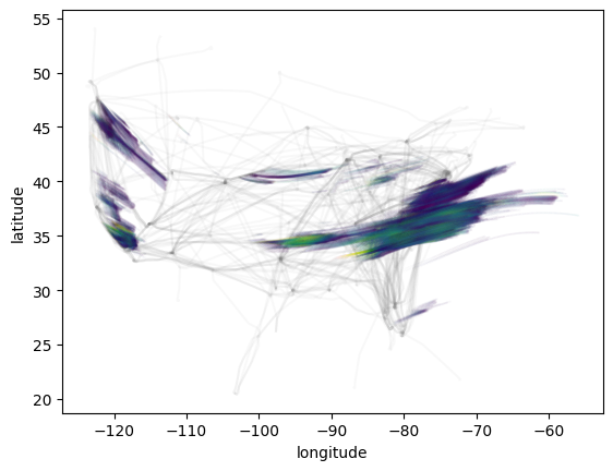
Visualize output¶

[13]:

ax = plt.subplot()
for flight in flights:
    flight.plot(ax=ax, color="gray", alpha=0.05)

contrail.plot.scatter(
    x="longitude",
    y="latitude",
    s=contrail["width"] / 100000,
    c=contrail["tau_contrail"],
    vmin=0,
    vmax=0.3,
    alpha=0.05,
    zorder=2,
    ax=ax,
);

../_images/notebooks_model-levels_22_0.png