Load GOES imagery

The ability to load and visualize GOES-16 was added in pycontrails 0.47.2. This notebook demonstrates basic usage.

import cartopy.crs as ccrs
import cartopy.feature as cfeature
import matplotlib.pyplot as plt

from pycontrails.datalib import goes

Download GOES data

By default, any GOES data will be cached on disk. Set cachestore=None to disable caching when defining the GOES object.

We download data for channels 1, 2, and 3. These are needed for creating a true color image.

handler = goes.GOES(region="conus", channels=("C01", "C02", "C03"))

# Download the data
da = handler.get("2023-02-05T18:00:00")
da

<xarray.DataArray 'CMI' (band_id: 3, y: 3000, x: 5000)>
dask.array<getitem, shape=(3, 3000, 5000), dtype=float32, chunksize=(1, 3000, 5000), chunktype=numpy.ndarray>
Coordinates:
    t                (band_id) datetime64[ns] 2023-02-05T18:02:35.739931008 ....
  * y                (y) float64 0.1282 0.1282 0.1282 ... 0.04428 0.04425
  * x                (x) float64 -0.1013 -0.1013 -0.1013 ... 0.0386 0.03863
    y_image          float32 0.08624
    x_image          float32 -0.03136
    band_wavelength  (band_id) float32 dask.array<chunksize=(1,), meta=np.ndarray>
  * band_id          (band_id) int32 1 2 3
Attributes:
    long_name:                  ABI L2+ Cloud and Moisture Imagery reflectanc...
    standard_name:              toa_lambertian_equivalent_albedo_multiplied_b...
    sensor_band_bit_depth:      10
    valid_range:                [   0 4095]
    units:                      1
    resolution:                 y: 0.000028 rad x: 0.000028 rad
    grid_mapping:               goes_imager_projection
    cell_methods:               t: point area: point
    ancillary_variables:        DQF
    goes_imager_projection:     {'long_name': 'GOES-R ABI fixed grid projecti...
    geospatial_lat_lon_extent:  {'long_name': 'geospatial latitude and longit...

xarray.DataArray

'CMI'

• band_id: 3
• y: 3000
• x: 5000

• dask.array<chunksize=(1, 3000, 5000), meta=np.ndarray>

  Array Chunk Bytes 171.66 MiB 57.22 MiB Shape (3, 3000, 5000) (1, 3000, 5000) Dask graph 3 chunks in 10 graph layers Data type float32 numpy.ndarray

• Coordinates: (7)
  • t
    (band_id)
    datetime64[ns]
    2023-02-05T18:02:35.739931008 .....

    long_name :

    J2000 epoch mid-point between the start and end image scan in seconds

    standard_name :

    time

    axis :

    T

    bounds :

    time_bounds

    array(['2023-02-05T18:02:35.739931008', '2023-02-05T18:02:35.738451968',
           '2023-02-05T18:02:35.739931008'], dtype='datetime64[ns]')

  • y
    (y)
    float64
    0.1282 0.1282 ... 0.04428 0.04425

    units :

    rad

    axis :

    Y

    long_name :

    GOES fixed grid projection y-coordinate

    standard_name :

    projection_y_coordinate

    array([0.128226, 0.128198, 0.12817 , ..., 0.04431 , 0.044282, 0.044254])

  • x
    (x)
    float64
    -0.1013 -0.1013 ... 0.0386 0.03863

    units :

    rad

    axis :

    X

    long_name :

    GOES fixed grid projection x-coordinate

    standard_name :

    projection_x_coordinate

    array([-0.101346, -0.101318, -0.10129 , ...,  0.03857 ,  0.038598,  0.038626])

  • y_image
    ()
    float32
    0.08624

    long_name :

    GOES-R fixed grid projection y-coordinate center of image

    standard_name :

    projection_y_coordinate

    units :

    rad

    axis :

    Y

    array(0.08624, dtype=float32)

  • x_image
    ()
    float32
    -0.03136

    long_name :

    GOES-R fixed grid projection x-coordinate center of image

    standard_name :

    projection_x_coordinate

    units :

    rad

    axis :

    X

    array(-0.03136, dtype=float32)

  • band_wavelength
    (band_id)
    float32
    dask.array<chunksize=(1,), meta=np.ndarray>

    long_name :

    ABI band central wavelength

    standard_name :

    sensor_band_central_radiation_wavelength

    units :

    um

    Array Chunk Bytes 12 B 4 B Shape (3,) (1,) Dask graph 3 chunks in 8 graph layers Data type float32 numpy.ndarray

  • band_id
    (band_id)
    int32
    1 2 3

    long_name :

    ABI band number

    standard_name :

    sensor_band_identifier

    units :

    1

    array([1, 2, 3], dtype=int32)

• Indexes: (3)
  • y
    PandasIndex

    PandasIndex(Index([ 0.12822599709033966,   0.1281979970899556,  0.12816999708957155,
             0.1281419970891875,  0.12811399708880344,   0.1280859970884194,
            0.12805799708803534,  0.12802999708765128,  0.12800199708726723,
            0.12797399708688317,
           ...
            0.04450599594201776,  0.04447799594163371, 0.044449995941249654,
             0.0444219959408656, 0.044393995940481545,  0.04436599594009749,
            0.04433799593971344,  0.04430999593932938,  0.04428199593894533,
           0.044253995938561275],
          dtype='float64', name='y', length=3000))

  • x
    PandasIndex

    PandasIndex(Index([-0.10134600102901459, -0.10131800102863053, -0.10129000102824648,
           -0.10126200102786242, -0.10123400102747837, -0.10120600102709432,
           -0.10117800102671026, -0.10115000102632621, -0.10112200102594215,
            -0.1010940010255581,
           ...
           0.038374000887415605,  0.03840200088779966,  0.03843000088818371,
            0.03845800088856777,  0.03848600088895182, 0.038514000889335875,
            0.03854200088971993, 0.038570000890103984,  0.03859800089048804,
            0.03862600089087209],
          dtype='float64', name='x', length=5000))

  • band_id
    PandasIndex

    PandasIndex(Index([1, 2, 3], dtype='int32', name='band_id'))

• Attributes: (11)

  long_name :

  ABI L2+ Cloud and Moisture Imagery reflectance factor

  standard_name :

  toa_lambertian_equivalent_albedo_multiplied_by_cosine_solar_zenith_angle

  sensor_band_bit_depth :

  10

  valid_range :

  [ 0 4095]

  units :

  1

  resolution :

  y: 0.000028 rad x: 0.000028 rad

  grid_mapping :

  goes_imager_projection

  cell_methods :

  t: point area: point

  ancillary_variables :

  DQF

  goes_imager_projection :

  {'long_name': 'GOES-R ABI fixed grid projection', 'grid_mapping_name': 'geostationary', 'perspective_point_height': 35786023.0, 'semi_major_axis': 6378137.0, 'semi_minor_axis': 6356752.31414, 'inverse_flattening': 298.2572221, 'latitude_of_projection_origin': 0.0, 'longitude_of_projection_origin': -75.0, 'sweep_angle_axis': 'x'}

  geospatial_lat_lon_extent :

  {'long_name': 'geospatial latitude and longitude references', 'geospatial_westbound_longitude': -152.10928, 'geospatial_northbound_latitude': 56.76145, 'geospatial_eastbound_longitude': -52.94688, 'geospatial_southbound_latitude': 14.57134, 'geospatial_lat_center': 30.083002, 'geospatial_lon_center': -87.096954, 'geospatial_lat_nadir': 0.0, 'geospatial_lon_nadir': -75.0, 'geospatial_lat_units': 'degrees_north', 'geospatial_lon_units': 'degrees_east'}

True color

First we plot a true color image of the CONUS region.

# Extract artifacts for plotting
rgb, src_crs, src_extent = goes.extract_goes_visualization(da, color_scheme="true")

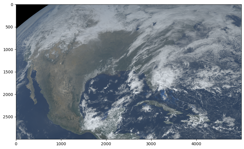
RGB array

The rgb array is a 3D array with shape (3, y, x). The first dimension contains the red, green, and blue channels, respectively. The second and third dimensions contain the y and x coordinates. The plot below shows the earth as seen by the satellite.

fig, ax = plt.subplots(figsize=(10, 10))
ax.imshow(rgb, origin="upper");

Projection artifacts

The src_crs is a cartopy.crs.Projection describing the coordinate reference system of the satellite data. The src_extent is a tuple containing the extent of the data in the source coordinate reference system. These can be used to plot the data on a map.

src_crs

<cartopy.crs.Geostationary object at 0x16ce0ac50>

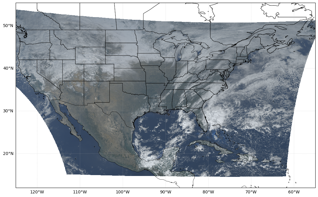
Visualize

We reproject the image to a Plate Carree projection and add state boundaries and coastlines to the plot.

dst_crs = ccrs.PlateCarree()

fig = plt.figure(figsize=(16, 8))
ax = fig.add_subplot(projection=dst_crs, extent=(-125, -55, 12, 50))
ax.coastlines(resolution="50m", color="black", linewidth=0.5)

# add state boundaries to plot
ax.add_feature(cfeature.STATES, edgecolor="black", linewidth=0.5)

ax.imshow(rgb, extent=src_extent, transform=src_crs, origin="upper", interpolation="none")

# Set the x and y ticks to use latitude and longitude labels
gl = ax.gridlines(draw_labels=True, alpha=0.5, linestyle=":")
gl.top_labels = False
gl.right_labels = False

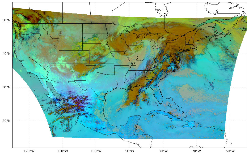
Ash color scheme

The ash color scheme was originally developed to visualize volcanic ash. It is also useful for visualizing contrails.

We download data for channels 11, 14, and 15 to create an ash color image.

handler = goes.GOES(region="conus", channels=("C11", "C14", "C15"))

# Download the data
da = handler.get("2023-02-09T18:00:00")

rgb, src_crs, src_extent = goes.extract_goes_visualization(da, color_scheme="ash")

fig = plt.figure(figsize=(16, 8))
ax = fig.add_subplot(projection=dst_crs, extent=(-125, -55, 12, 50))
ax.coastlines(resolution="50m", color="black", linewidth=0.5)

# add state boundaries to plot
ax.add_feature(cfeature.STATES, edgecolor="black", linewidth=0.5)

ax.imshow(rgb, extent=src_extent, transform=src_crs, origin="upper", interpolation="none")

# Set the x and y ticks to use latitude and longitude labels
gl = ax.gridlines(draw_labels=True, alpha=0.5, linestyle=":")
gl.top_labels = False
gl.right_labels = False