ACCF¶

Interface to the ACCF (algorithmic climate change functions) from the DLR library climaccf.

References¶

Dietmüller, Simone. “Dlr-Pa/Climaccf: Dataset Update for GMDD.” Zenodo, September 13, 2022. https://doi.org/10.5281/zenodo.7074582.
Dietmüller, Simone, Sigrun Matthes, Katrin Dahlmann, Hiroshi Yamashita, Abolfazl Simorgh, Manuel Soler, Florian Linke, et al. “A Python Library for Computing Individual and Merged Non-CO2 Algorithmic Climate Change Functions: CLIMaCCF V1.0.” Preprint. Atmospheric sciences, October 17, 2022. https://doi.org/10.5194/gmd-2022-203.

[1]:

import numpy as np
import pandas as pd
import matplotlib.pyplot as plt

from pycontrails import Flight
from pycontrails.datalib.ecmwf import ERA5
from pycontrails.models.accf import ACCF
from pycontrails.physics import units

Set Domain¶

time / altitude

[2]:

time_bounds = ("2022-01-01 12:00:00", "2022-01-01 15:00:00")
pressure_levels = [200, 225, 250]

Download meteorology data from ECMWF¶

This demo uses ERA5 via the Copernicus Data Store (CDS) for met data. This requires account with Copernicus Data Portal and local ~/.cdsapirc file with credentials.

[3]:

# pressure level data
era5_pl = ERA5(
    time=time_bounds,
    variables=[
        "air_temperature",
        "specific_humidity",
        "potential_vorticity",
        "geopotential",
        "relative_humidity",
        "northward_wind",
        "eastward_wind",
    ],
    pressure_levels=pressure_levels,
)

# single level data (radiation)
era5_sl = ERA5(
    time=time_bounds,
    variables=["surface_solar_downward_radiation", "top_net_thermal_radiation"],
)

pl = era5_pl.open_metdataset()
sl = era5_sl.open_metdataset()

Create example flight¶

[4]:

# Note: ACCF output is in K/kg of fuel so you will need to provide fuel burn of the flight to get impact in K
n = 10000
longitude = np.linspace(45, 58, n) + np.linspace(0, 1, n)
latitude = np.linspace(45, 54, n) - np.linspace(0, 1, n)
altitude = units.pl_to_m(225) * np.ones(n)

start = np.datetime64(time_bounds[0])
end = start + np.timedelta64(90, "m")  # 90 minute flight
time = pd.date_range(start, end, periods=n)
fl = Flight(
    longitude=longitude,
    latitude=latitude,
    altitude=altitude,
    time=time,
    aircraft_type="B737",
    flight_id=17,
)
fl["fuel_flow"] = np.linspace(2.1, 2.4, n)  # kg/s

[5]:

fl

[5]:

Flight [5 keys x 10000 length, 3 attributes]

Attributes
time	[2022-01-01 12:00:00, 2022-01-01 13:30:00]
longitude	[45.0, 59.0]
latitude	[45.0, 53.0]
altitude	[11037.0, 11037.0]
aircraft_type	B737
flight_id	17
crs	EPSG:4326

	longitude	latitude	time	altitude	fuel_flow
0	45.000000	45.0000	2022-01-01 12:00:00.000000000	11037.01126	2.10000
1	45.001400	45.0008	2022-01-01 12:00:00.540054005	11037.01126	2.10003
2	45.002800	45.0016	2022-01-01 12:00:01.080108010	11037.01126	2.10006
3	45.004200	45.0024	2022-01-01 12:00:01.620162016	11037.01126	2.10009
4	45.005601	45.0032	2022-01-01 12:00:02.160216021	11037.01126	2.10012
...	...	...	...	...	...
9995	58.994399	52.9968	2022-01-01 13:29:57.839783978	11037.01126	2.39988
9996	58.995800	52.9976	2022-01-01 13:29:58.379837983	11037.01126	2.39991
9997	58.997200	52.9984	2022-01-01 13:29:58.919891989	11037.01126	2.39994
9998	58.998600	52.9992	2022-01-01 13:29:59.459945994	11037.01126	2.39997
9999	59.000000	53.0000	2022-01-01 13:30:00.000000000	11037.01126	2.40000

10000 rows × 5 columns

Initialize ACCF model and evaluate on flight¶

[7]:

ac = ACCF(met=pl, surface=sl)

[8]:

# Evaluate ACCFs over this flight
fl = ac.eval(fl)

selected forecast step:  6.0 HR

 UserWarning: For this configuration formation of persistent contrails is possible, if temperatures are low enough (below 235K) and relative humidity (with respect to ice) is above or at 90.0%. However keep in mind that the threshold value for the relative humidity varies with the used forecast model and its resolution. In order to choose the appropriate threshold value, you should read the details given in Section 5.1 of the connected publication of Dietmueller et al. 2022

Explore the output¶

Raw output:

[9]:

fl

[9]:

Flight [27 keys x 10000 length, 7 attributes]

Attributes
time	[2022-01-01 12:00:00, 2022-01-01 13:30:00]
longitude	[45.0, 59.0]
latitude	[45.0, 53.0]
altitude	[11037.0, 11037.0]
aircraft_type	B737
flight_id	17
crs	EPSG:4326
met_source_provider	ECMWF
met_source_dataset	ERA5
met_source_product	reanalysis
pycontrails_version	0.47.3.dev86

	longitude	latitude	time	altitude	fuel_flow	flight_id	air_temperature	specific_humidity	potential_vorticity	geopotential	...	aCCF_CH4	aCCF_O3	aCCF_H2O	aCCF_nCont	aCCF_dCont	aCCF_Cont	aCCF_CO2	aCCF_merged	aCCF_NOx	Fin
0	45.000000	45.0000	2022-01-01 12:00:00.000000000	11037.01126	2.10000	17.0	215.779129	0.000007	0.000007	105447.960938	...	-4.455085e-13	1.637062e-12	7.799343e-16	0.000000e+00	-0.000000e+00	0.000000e+00	6.940000e-16	1.696413e-14	1.191553e-12	509.002230
1	45.001400	45.0008	2022-01-01 12:00:00.540054005	11037.01126	2.10003	17.0	215.779785	0.000007	0.000007	105447.773438	...	-4.455091e-13	1.637061e-12	7.799481e-16	0.000000e+00	-0.000000e+00	0.000000e+00	6.940000e-16	1.696413e-14	1.191552e-12	508.984589
2	45.002800	45.0016	2022-01-01 12:00:01.080108010	11037.01126	2.10006	17.0	215.780441	0.000007	0.000007	105447.578125	...	-4.455098e-13	1.637061e-12	7.799622e-16	0.000000e+00	-0.000000e+00	0.000000e+00	6.940000e-16	1.696412e-14	1.191551e-12	508.966947
3	45.004200	45.0024	2022-01-01 12:00:01.620162016	11037.01126	2.10009	17.0	215.781097	0.000007	0.000007	105447.390625	...	-4.455104e-13	1.637060e-12	7.799766e-16	0.000000e+00	-0.000000e+00	0.000000e+00	6.940000e-16	1.696412e-14	1.191550e-12	508.949306
4	45.005601	45.0032	2022-01-01 12:00:02.160216021	11037.01126	2.10012	17.0	215.781754	0.000007	0.000007	105447.195312	...	-4.455110e-13	1.637060e-12	7.799912e-16	0.000000e+00	-0.000000e+00	0.000000e+00	6.940000e-16	1.696412e-14	1.191549e-12	508.931664
...	...	...	...	...	...	...	...	...	...	...	...	...	...	...	...	...	...	...	...	...	...
9995	58.994399	52.9968	2022-01-01 13:29:57.839783978	11037.01126	2.39988	17.0	209.364670	0.000013	0.000007	104271.609375	...	-4.495710e-13	1.523755e-12	7.788148e-16	1.717789e-28	-1.052829e-27	1.717789e-28	6.940000e-16	1.543721e-14	1.074184e-12	328.603173
9996	58.995800	52.9976	2022-01-01 13:29:58.379837983	11037.01126	2.39991	17.0	209.364761	0.000013	0.000007	104271.421875	...	-4.495715e-13	1.523748e-12	7.789030e-16	1.717655e-28	-1.052830e-27	1.717655e-28	6.940000e-16	1.543720e-14	1.074177e-12	328.584764
9997	58.997200	52.9984	2022-01-01 13:29:58.919891989	11037.01126	2.39994	17.0	209.364868	0.000013	0.000007	104271.234375	...	-4.495719e-13	1.523742e-12	7.789914e-16	1.717522e-28	-1.052832e-27	1.717522e-28	6.940000e-16	1.543720e-14	1.074170e-12	328.566356
9998	58.998600	52.9992	2022-01-01 13:29:59.459945994	11037.01126	2.39997	17.0	209.364960	0.000013	0.000007	104271.046875	...	-4.495724e-13	1.523735e-12	7.790802e-16	1.717388e-28	-1.052834e-27	1.717388e-28	6.940000e-16	1.543720e-14	1.074163e-12	328.547947
9999	59.000000	53.0000	2022-01-01 13:30:00.000000000	11037.01126	2.40000	17.0	209.365051	0.000013	0.000007	104270.859375	...	-4.495728e-13	1.523728e-12	7.791693e-16	1.717254e-28	-1.052836e-27	1.717254e-28	6.940000e-16	1.543719e-14	1.074156e-12	328.529539

10000 rows × 27 columns

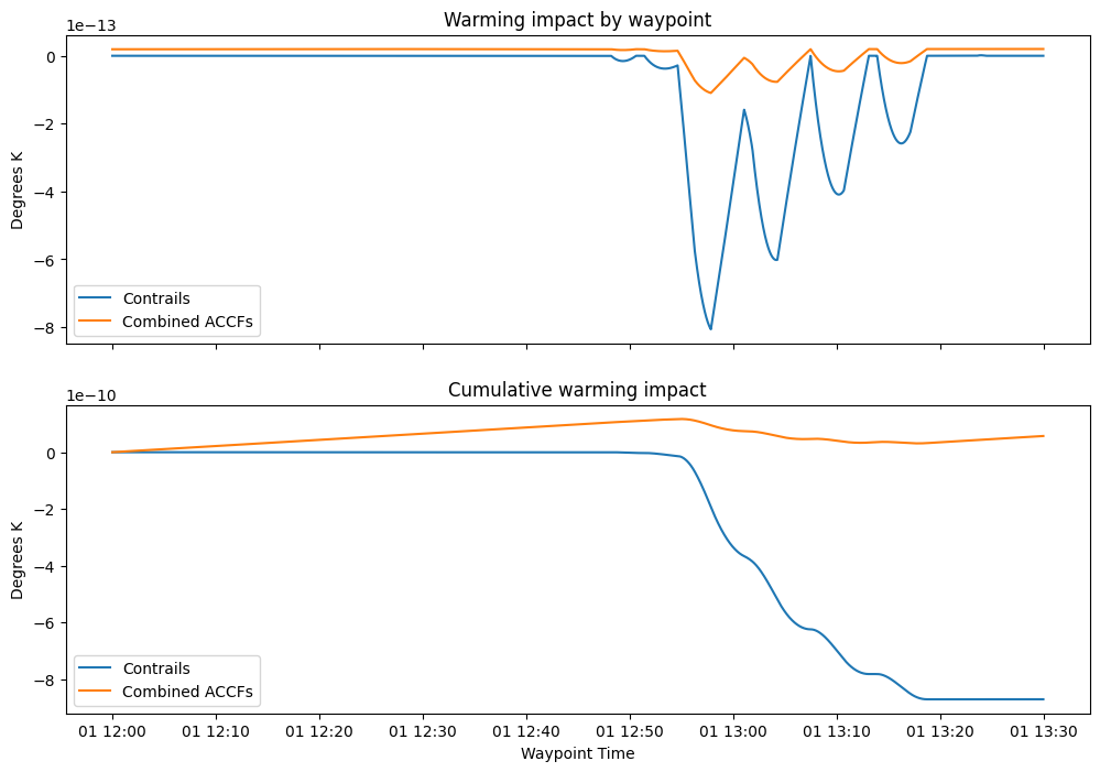
Now convert fuel flow to total fuel burned by waypoint, and get the impact of each flight waypoint and plot

[11]:

# Waypoint duration in seconds
dt_sec = fl.segment_duration()

# kg fuel per contrail
fuel_burn = fl["fuel_flow"] * dt_sec

# Get impacts in degrees K per waypoint
warming_contrails = fuel_burn * fl["aCCF_Cont"]
warming_merged = fuel_burn * fl["aCCF_merged"]

[12]:

f, (ax0, ax1) = plt.subplots(2, 1, sharex=True, figsize=(12, 8))
ax0.plot(fl["time"], warming_contrails, label="Contrails")
ax0.plot(fl["time"], warming_merged, label="Combined ACCFs")
ax0.set_ylabel("Degrees K")
ax0.set_title("Warming impact by waypoint")
ax0.legend()

ax1.plot(fl["time"], np.cumsum(warming_contrails), label="Contrails")
ax1.plot(fl["time"], np.cumsum(warming_merged), label="Combined ACCFs")
ax1.legend()
ax1.set_xlabel("Waypoint Time")
ax1.set_ylabel("Degrees K")
ax1.set_title("Cumulative warming impact");

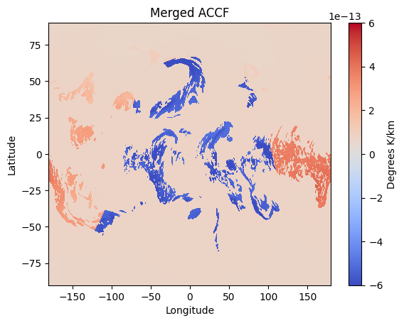
Grid ACCF with Parameters¶

[13]:

ac = ACCF(pl, sl, {"emission_scenario": "future_scenario", "accf_v": "V1.1"})
ds = ac.eval()  # This will evaluate over the met grid

selected forecast step:  6.0 HR

 UserWarning: For this configuration formation of persistent contrails is possible, if temperatures are low enough (below 235K) and relative humidity (with respect to ice) is above or at 90.0%. However keep in mind that the threshold value for the relative humidity varies with the used forecast model and its resolution. In order to choose the appropriate threshold value, you should read the details given in Section 5.1 of the connected publication of Dietmueller et al. 2022

[14]:

fig, ax = plt.subplots()
p = ax.pcolor(
    ds["longitude"].data,
    ds["latitude"].data,
    ds["aCCF_merged"].data[:, :, 0, 0].T,
    cmap="coolwarm",
    vmin=-6e-13,
    vmax=6e-13,
)
ax.set_xlabel("Longitude")
ax.set_ylabel("Latitude")
ax.set_title("Merged ACCF")
cbar = plt.colorbar(p)
cbar.set_label("Degrees K/km");