Schmidt-Appleman criterion
Model areas of the atmosphere that satisfy the Schmidt-Appleman criterion (SAC).
Met Data
Requires account with Copernicus Data Portal and local
~/.cdsapirc filewith credentials.
[1]:
# ignore pycontrails warning about ECMWF humidity scaling
import warnings

import pandas as pd

from pycontrails import Flight
from pycontrails.datalib.ecmwf import ERA5
from pycontrails.models.sac import SAC

warnings.filterwarnings(message=r"[\s\S]* humidity scaling [\s\S]*", action="ignore")
Get Data
[2]:
time = ("2022-03-01 00:00:00", "2022-03-01 03:00:00")
pressure_levels = [300, 250, 200]
variables = ["t", "q"]  # only temperature and humidity are needed for SAC
[3]:
era5 = ERA5(time=time, variables=variables, pressure_levels=pressure_levels)
met = era5.open_metdataset()
Calculations
[4]:
# evaluate SAC on met grid
sac_mds = SAC(met=met).eval()  # returns a MetDataset
sac = sac_mds["sac"]  # extract the SAC MetDataArray

# edge detection algorithm using differentiation to reduce the areas to lines
sac_edges = sac.find_edges()
Figures
[5]:
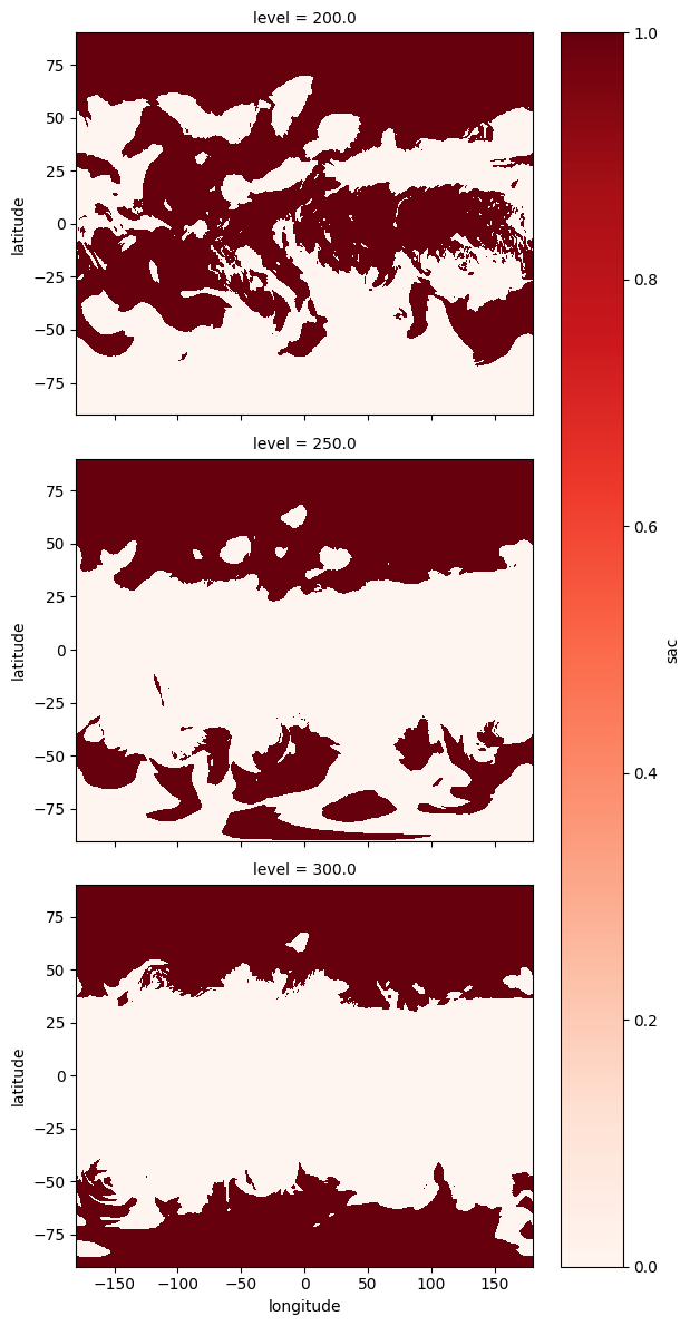
# plot sac regions for each pressure level
da = sac.data.isel(time=0)
da.plot(x="longitude", y="latitude", row="level", cmap="Reds", figsize=(6, 12));
[6]:
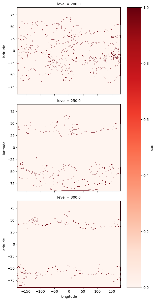
# plot issr edges for each pressure level
da = sac_edges.data.isel(time=0)
da.plot(x="longitude", y="latitude", row="level", cmap="Reds", figsize=(6, 12));
Interpolate
Run model along a flight path
[7]:
# Load flight
df = pd.read_csv("data/flight.csv", parse_dates=["time"])
fl = Flight(data=df, flight_id="acdd1b", callsign="AAL1158")
[8]:
# run model for across full input domain
# outputs global ice super-saturated regions as 1, all other regions as 0
# np.nan is returned outside of the met domain
fl_out = SAC(met).eval(source=fl)
fl_out["sac"]
[8]:
array([nan, nan,  1., nan, nan, nan, nan, nan, nan, nan, nan, nan, nan,
        1.,  1.,  1.,  1.,  1.,  1.,  1.,  1.,  1.,  1.,  1.,  1.,  1.,
        1.,  1.,  1.,  1.,  1.,  1.,  1.,  1.,  1.,  1.,  1.,  1.,  1.,
        1.,  1.,  1.,  1.,  1.,  1.,  1.,  1.,  1.,  1.,  1.,  1.,  1.,
        1.,  1.,  1.,  1.,  1.,  1.,  1.,  1.,  1.,  1.,  1.,  1.,  1.,
        1.,  1.,  1.,  1.,  1.,  1.,  1.,  1.,  1.,  1.,  1.,  1.,  1.,
        1.,  1.,  1.,  1.,  1.,  1.,  1.,  1.,  1.,  1.,  1.,  1.,  1.,
        1.,  1.,  1.,  1.,  1.,  1.,  1.,  1.,  1.,  1.,  1.,  1.,  1.,
        1.,  1.,  1.,  1.,  1.,  1.,  1.,  1.,  1.,  1.,  1.,  1.,  1.,
        1.,  1.,  1.,  1.,  1.,  1.,  1.,  1.,  1.,  1.,  1., nan, nan,
       nan, nan, nan, nan, nan, nan, nan, nan, nan, nan, nan, nan, nan,
       nan, nan, nan, nan, nan, nan, nan, nan, nan, nan, nan, nan, nan,
       nan, nan, nan, nan, nan, nan, nan, nan, nan, nan, nan, nan, nan,
       nan, nan, nan, nan, nan, nan])
[9]:
# Get the length of the Flight in the SAC region
fl_out.length_met("sac")
[9]:
1390898.4268105943
[10]:
# The SAC is sensitive to the engine efficiency of the aircraft.
# As this value decreases, fewer waypoints satisfy the SAC.
fl_out = SAC(met, engine_efficiency=0.0).eval(source=fl)
fl_out["sac"]
[10]:
array([nan, nan,  0., nan, nan, nan, nan, nan, nan, nan, nan, nan, nan,
        0.,  1.,  1.,  1.,  1.,  1.,  0.,  0.,  0.,  0.,  0.,  1.,  1.,
        1.,  1.,  1.,  1.,  1.,  1.,  1.,  1.,  1.,  1.,  1.,  1.,  1.,
        1.,  1.,  1.,  1.,  1.,  1.,  1.,  1.,  1.,  1.,  1.,  1.,  1.,
        1.,  1.,  1.,  1.,  1.,  1.,  1.,  1.,  1.,  1.,  1.,  1.,  1.,
        1.,  1.,  1.,  1.,  1.,  1.,  1.,  1.,  1.,  1.,  1.,  1.,  1.,
        1.,  1.,  1.,  1.,  1.,  1.,  1.,  1.,  1.,  1.,  1.,  1.,  1.,
        1.,  1.,  1.,  1.,  1.,  1.,  1.,  1.,  1.,  1.,  1.,  1.,  1.,
        1.,  1.,  1.,  1.,  1.,  1.,  1.,  1.,  1.,  1.,  1.,  1.,  1.,
        1.,  1.,  1.,  1.,  1.,  1.,  1.,  1.,  1.,  1.,  1., nan, nan,
       nan, nan, nan, nan, nan, nan, nan, nan, nan, nan, nan, nan, nan,
       nan, nan, nan, nan, nan, nan, nan, nan, nan, nan, nan, nan, nan,
       nan, nan, nan, nan, nan, nan, nan, nan, nan, nan, nan, nan, nan,
       nan, nan, nan, nan, nan, nan])