CoCiP
Contrail Cirrus Predicition (CoCiP) model evaluation along a flight trajectory.
References
Schumann, U. “A Contrail Cirrus Prediction Model.” Geoscientific Model Development 5, no. 3 (May 3, 2012): 543–80. https://doi.org/10.5194/gmd-5-543-2012.
Schumann, U., B. Mayer, K. Graf, and H. Mannstein. “A Parametric Radiative Forcing Model for Contrail Cirrus.” Journal of Applied Meteorology and Climatology 51, no. 7 (July 2012): 1391–1406. https://doi.org/10.1175/JAMC-D-11-0242.1.
Schumann, Ulrich, Robert Baumann, Darrel Baumgardner, Sarah T. Bedka, David P. Duda, Volker Freudenthaler, Jean-Francois Gayet, et al. 2017. “Properties of Individual Contrails: A Compilation of Observations and Some Comparisons.” Atmospheric Chemistry and Physics 17 (1): 403–38. https://doi.org/10.5194/acp-17-403-2017.
Teoh, Roger, Ulrich Schumann, Arnab Majumdar, and Marc E. J. Stettler. “Mitigating the Climate Forcing of Aircraft Contrails by Small-Scale Diversions and Technology Adoption.” Environmental Science & Technology 54, no. 5 (March 3, 2020): 2941–50. https://doi.org/10.1021/acs.est.9b05608.
Teoh, Roger, Ulrich Schumann, Edward Gryspeerdt, Marc Shapiro, Jarlath Molloy, George Koudis, Christiane Voigt, and Marc E. J. Stettler. 2022. “Aviation Contrail Climate Effects in the North Atlantic from 2016 to 2021.” Atmospheric Chemistry and Physics 22 (16): 10919–35. https://doi.org/10.5194/acp-22-10919-2022.
Teoh, Roger, Ulrich Schumann, Christiane Voigt, Tobias Schripp, Marc Shapiro, Zebediah Engberg, Jarlath Molloy, George Koudis, and Marc E. J. Stettler. 2022. “Targeted Use of Sustainable Aviation Fuel to Maximize Climate Benefits.” Environmental Science & Technology, November. https://doi.org/10.1021/acs.est.2c05781.
[1]:
import numpy as np
import pandas as pd
from matplotlib import pyplot as plt

from pycontrails import Flight, MetDataset
from pycontrails.datalib.ecmwf import ERA5
from pycontrails.models.cocip import Cocip
from pycontrails.models.humidity_scaling import ConstantHumidityScaling

plt.rcParams["figure.figsize"] = (10, 6)
Download meteorology data from ECMWF
This demo uses ERA5 via the Copernicus Data Store (CDS) for met data. This requires account with Copernicus Data Portal and local ~/.cdsapirc file with credentials.
Note this will download ~1 GB of meteorology data to your computer
[2]:
time_bounds = ("2022-03-01 00:00:00", "2022-03-01 23:00:00")
pressure_levels = (300, 250, 200)
[3]:
era5pl = ERA5(
    time=time_bounds,
    variables=Cocip.met_variables + Cocip.optional_met_variables,
    pressure_levels=pressure_levels,
)
era5sl = ERA5(time=time_bounds, variables=Cocip.rad_variables)
[4]:
# download data from ERA5 (or open from cache)
met = era5pl.open_metdataset()
rad = era5sl.open_metdataset()
Load Flight Data
Flight can be loaded from CSV, parquet, or created from a pandas DataFrame
[5]:
# demo synthetic flight
flight_attrs = {
    "flight_id": "test",
    # set constants along flight path
    "true_airspeed": 226.099920796651,  # true airspeed, m/s
    "thrust": 0.22,  # thrust_setting
    "nvpm_ei_n": 1.897462e15,  # non-volatile emissions index
    "aircraft_type": "E190",
    "wingspan": 48,  # m
    "n_engine": 2,
}

# Example flight
df = pd.DataFrame()
df["longitude"] = np.linspace(-25, -40, 100)
df["latitude"] = np.linspace(34, 40, 100)
df["altitude"] = np.linspace(10900, 10900, 100)
df["engine_efficiency"] = np.linspace(0.34, 0.35, 100)
df["fuel_flow"] = np.linspace(2.1, 2.4, 100)  # kg/s
df["aircraft_mass"] = np.linspace(154445, 154345, 100)  # kg
df["time"] = pd.date_range("2022-03-01T00:15:00", "2022-03-01T02:30:00", periods=100)

flight = Flight(df, attrs=flight_attrs)
flight
[5]:
| Attributes | |
|---|---|
| time | [2022-03-01 00:15:00, 2022-03-01 02:30:00] |
| longitude | [-40.0, -25.0] |
| latitude | [34.0, 40.0] |
| altitude | [10900.0, 10900.0] |
| flight_id | test |
| true_airspeed | 226.099920796651 |
| thrust | 0.22 |
| nvpm_ei_n | 1897462000000000.0 |
| aircraft_type | E190 |
| wingspan | 48 |
| n_engine | 2 |
| crs | EPSG:4326 |
| longitude | latitude | altitude | engine_efficiency | fuel_flow | aircraft_mass | time | |
|---|---|---|---|---|---|---|---|
| 0 | -25.000000 | 34.000000 | 10900.0 | 0.340000 | 2.100000 | 154445.000000 | 2022-03-01 00:15:00.000000000 |
| 1 | -25.151515 | 34.060606 | 10900.0 | 0.340101 | 2.103030 | 154443.989899 | 2022-03-01 00:16:21.818181818 |
| 2 | -25.303030 | 34.121212 | 10900.0 | 0.340202 | 2.106061 | 154442.979798 | 2022-03-01 00:17:43.636363636 |
| 3 | -25.454545 | 34.181818 | 10900.0 | 0.340303 | 2.109091 | 154441.969697 | 2022-03-01 00:19:05.454545454 |
| 4 | -25.606061 | 34.242424 | 10900.0 | 0.340404 | 2.112121 | 154440.959596 | 2022-03-01 00:20:27.272727272 |
| ... | ... | ... | ... | ... | ... | ... | ... |
| 95 | -39.393939 | 39.757576 | 10900.0 | 0.349596 | 2.387879 | 154349.040404 | 2022-03-01 02:24:32.727272727 |
| 96 | -39.545455 | 39.818182 | 10900.0 | 0.349697 | 2.390909 | 154348.030303 | 2022-03-01 02:25:54.545454545 |
| 97 | -39.696970 | 39.878788 | 10900.0 | 0.349798 | 2.393939 | 154347.020202 | 2022-03-01 02:27:16.363636363 |
| 98 | -39.848485 | 39.939394 | 10900.0 | 0.349899 | 2.396970 | 154346.010101 | 2022-03-01 02:28:38.181818181 |
| 99 | -40.000000 | 40.000000 | 10900.0 | 0.350000 | 2.400000 | 154345.000000 | 2022-03-01 02:30:00.000000000 |
100 rows × 7 columns
Run Cocip on a single flight
In this first example, the Flight has aircraft performance (i.e. nvpm_ei_n) hardcoded into the data as constants. This data is assumed to be constant at every flight waypoint.
Caveat
When the
Cocipmodel is run on oneFlight, the default behavior is to downselect the meteorology to a region surrounding the flight and process the meteorology (i.e. humidity scaling,tau_cirrus) on the smaller domain. The implications of this processing is each instance of a single-flightCocipmodel should only be run once.We ignore the warning here about humidity scaling for ECMWF data sources
[6]:
params = {
    "dt_integration": np.timedelta64(10, "m"),
    # The humidity_scaling parameter is only used for ECMWF ERA5 data
    # based on Teoh 2020 and Teoh 2022 - https://acp.copernicus.org/preprints/acp-2022-169/acp-2022-169.pdf
    # Here we use an example of constantly scaling the humidity value by 0.99
    "humidity_scaling": ConstantHumidityScaling(rhi_adj=0.99),
}
cocip = Cocip(met=met, rad=rad, params=params)
[7]:
output_flight = cocip.eval(source=flight)
Explore Flight Output
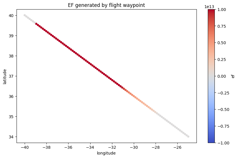
The output_flight object holds roughly 50 variables of interest. The energy forcing ef field is a primary model output. Waypoints not producing persistent contrails are assigned an ef value of 0.
[8]:
df = output_flight.dataframe
df.head()
[8]:
| waypoint | longitude | latitude | altitude | engine_efficiency | fuel_flow | aircraft_mass | time | flight_id | level | ... | n_ice_per_m_1 | ef | contrail_age | sdr_mean | rsr_mean | olr_mean | rf_sw_mean | rf_lw_mean | rf_net_mean | cocip | |
|---|---|---|---|---|---|---|---|---|---|---|---|---|---|---|---|---|---|---|---|---|---|
| 0 | 0 | -25.000000 | 34.000000 | 10900.0 | 0.340000 | 2.100000 | 154445.000000 | 2022-03-01 00:15:00.000000000 | test | 229.908663 | ... | 1.211936e+13 | 0.0 | 0 days | NaN | NaN | NaN | NaN | NaN | NaN | 0.0 |
| 1 | 1 | -25.151515 | 34.060606 | 10900.0 | 0.340101 | 2.103030 | 154443.989899 | 2022-03-01 00:16:21.818181818 | test | 229.908663 | ... | 1.299153e+13 | 0.0 | 0 days | NaN | NaN | NaN | NaN | NaN | NaN | 0.0 |
| 2 | 2 | -25.303030 | 34.121212 | 10900.0 | 0.340202 | 2.106061 | 154442.979798 | 2022-03-01 00:17:43.636363636 | test | 229.908663 | ... | 1.363941e+13 | 0.0 | 0 days | NaN | NaN | NaN | NaN | NaN | NaN | 0.0 |
| 3 | 3 | -25.454545 | 34.181818 | 10900.0 | 0.340303 | 2.109091 | 154441.969697 | 2022-03-01 00:19:05.454545454 | test | 229.908663 | ... | 1.410562e+13 | 0.0 | 0 days | NaN | NaN | NaN | NaN | NaN | NaN | 0.0 |
| 4 | 4 | -25.606061 | 34.242424 | 10900.0 | 0.340404 | 2.112121 | 154440.959596 | 2022-03-01 00:20:27.272727272 | test | 229.908663 | ... | 1.438106e+13 | 0.0 | 0 days | NaN | NaN | NaN | NaN | NaN | NaN | 0.0 |
5 rows × 45 columns
[9]:
df.plot.scatter(
    x="longitude",
    y="latitude",
    c="ef",
    cmap="coolwarm",
    vmin=-1e13,
    vmax=1e13,
    title="EF generated by flight waypoint",
);
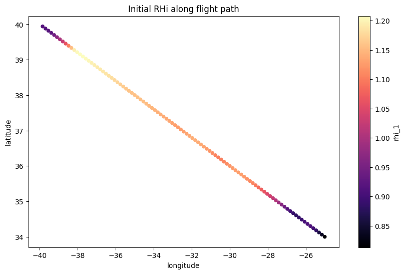
[10]:
df.plot.scatter(
    x="longitude",
    y="latitude",
    c="rhi_1",
    cmap="magma",
    title="Initial RHi along flight path",
);
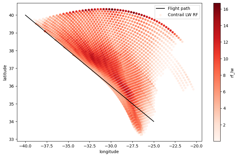
Explore Contrail Output
The
cocip.contrailattribute is a`pandas.DataFrame<https://pandas.pydata.org/pandas-docs/stable/reference/api/pandas.DataFrame.html>`__ representation of the contrail waypoints.
[11]:
contrail = cocip.contrail
contrail.head()
[11]:
| waypoint | flight_id | formation_time | time | age | longitude | latitude | altitude | level | continuous | ... | tau_contrail | dn_dt_agg | dn_dt_turb | rf_sw | rf_lw | rf_net | persistent | ef | timestep | age_hours | |
|---|---|---|---|---|---|---|---|---|---|---|---|---|---|---|---|---|---|---|---|---|---|
| 0 | 16 | test | 2022-03-01 00:36:49.090909090 | 2022-03-01 00:40:00 | 0 days 00:03:10.909090910 | -27.378049 | 34.922418 | 10855.165152 | 231.533890 | True | ... | 0.058053 | 7.476665e-20 | 0.000051 | 0.0 | 0.555465 | 0.555465 | True | 1.099225e+09 | 2 | 0.053030 |
| 1 | 17 | test | 2022-03-01 00:38:10.909090909 | 2022-03-01 00:40:00 | 0 days 00:01:49.090909091 | -27.548832 | 35.003469 | 10855.511035 | 231.521316 | True | ... | 0.165581 | 2.538742e-19 | 0.000077 | 0.0 | 1.976229 | 1.976229 | True | 9.428853e+08 | 2 | 0.030303 |
| 2 | 18 | test | 2022-03-01 00:39:32.727272727 | 2022-03-01 00:40:00 | 0 days 00:00:00 | -27.720407 | 35.084249 | 10855.340639 | 231.527510 | False | ... | 0.408836 | 4.056703e-19 | 0.000233 | 0.0 | 4.600390 | 4.600390 | True | 0.000000e+00 | 2 | 0.000000 |
| 0 | 17 | test | 2022-03-01 00:38:10.909090909 | 2022-03-01 00:50:00 | 0 days 00:11:49.090909091 | -27.401596 | 34.855488 | 10855.704079 | 231.514299 | True | ... | 0.036824 | 9.873238e-20 | 0.000026 | 0.0 | 0.561865 | 0.561865 | True | 7.060254e+09 | 3 | 0.196970 |
| 1 | 18 | test | 2022-03-01 00:39:32.727272727 | 2022-03-01 00:50:00 | 0 days 00:10:27.272727273 | -27.569577 | 34.937639 | 10857.240565 | 231.458453 | True | ... | 0.047199 | 2.494850e-19 | 0.000030 | 0.0 | 0.854236 | 0.854236 | True | 8.330392e+09 | 3 | 0.174242 |
5 rows × 56 columns
[12]:
ax = plt.axes()

cocip.source.dataframe.plot(
    "longitude",
    "latitude",
    color="k",
    ax=ax,
    label="Flight path",
)
cocip.contrail.plot.scatter(
    "longitude",
    "latitude",
    c="rf_lw",
    cmap="Reds",
    ax=ax,
    label="Contrail LW RF",
)
ax.legend();
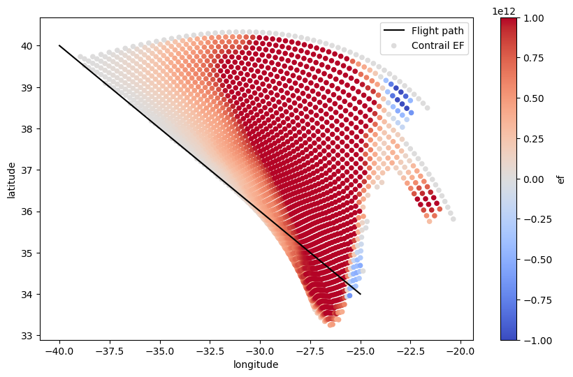
[13]:
ax = plt.axes()

cocip.source.dataframe.plot(
    "longitude",
    "latitude",
    color="k",
    ax=ax,
    label="Flight path",
)
cocip.contrail.plot.scatter(
    "longitude",
    "latitude",
    c="ef",
    cmap="coolwarm",
    vmin=-1e12,
    vmax=1e12,
    ax=ax,
    label="Contrail EF",
)
ax.legend();
Explore Flight Summary
A curated set of statistics available after a Flight has been run through eval
[14]:
from pycontrails.models.cocip import (
    contrail_flight_summary_statistics,
    flight_waypoint_summary_statistics,
)
[15]:
# flight_statistics = cocip.output_flight_statistics()
# flight_statistics

waypoint_summary = flight_waypoint_summary_statistics(cocip.source, cocip.contrail)
flight_summary = contrail_flight_summary_statistics(waypoint_summary)
flight_summary
[15]:
| flight_id | total_flight_distance_flown | total_contrails_formed | total_persistent_contrails_formed | mean_lifetime_contrail_altitude | mean_lifetime_rhi | mean_lifetime_n_ice_per_m | mean_lifetime_r_ice_vol | mean_lifetime_contrail_width | mean_lifetime_contrail_depth | ... | mean_lifetime_tau_cirrus | mean_contrail_lifetime | max_contrail_lifetime | mean_lifetime_rf_sw | mean_lifetime_rf_lw | mean_lifetime_rf_net | total_energy_forcing | mean_lifetime_olr | mean_lifetime_sdr | mean_lifetime_rsr | |
|---|---|---|---|---|---|---|---|---|---|---|---|---|---|---|---|---|---|---|---|---|---|
| 0 | test | 1.489373e+06 | 1.489373e+06 | 1.489373e+06 | 10924.967627 | 1.115407 | 9.352614e+12 | 0.000006 | 15384.899335 | 535.5604 | ... | 0.251802 | 5.364979 | 10.583333 | -0.157952 | 5.550725 | 5.392773 | 2.340121e+15 | 192.821976 | 22.198721 | 9.819747 |
1 rows × 21 columns
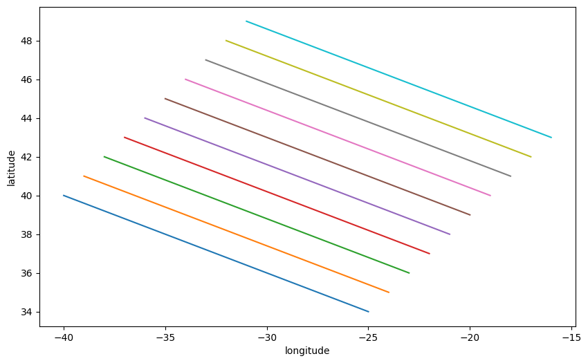
Run Cocip on Multiple Flights
Run multiple Flight inputs on a single set of meteorology.
For this demo, we’ll copy the original flight and tweak its longitude and latitudes values.
[16]:
flights = []
for i in range(10):
    fl = flight.copy()
    fl.attrs.update(flight_id=f"test-{i:02d}")
    fl.update(latitude=flight["latitude"] + i)
    fl.update(longitude=flight["longitude"] + i)
    flights.append(fl)
[17]:
# Visualize the fleet of 10 flights
ax = plt.axes()
for fl in flights:
    fl.plot(ax=ax)
Run the Cocip model over a list[Flight] objects
[18]:
cocip = Cocip(
    met=met,
    rad=rad,
    process_emissions=False,
    humidity_scaling=ConstantHumidityScaling(rhi_adj=0.99),
)

# returns list of Flight outputs
output_flights = cocip.eval(source=flights)
[19]:
# print EF for each flight
for fl in output_flights:
    print(f"{fl.attrs['flight_id']}: {np.sum(fl['ef'])}")
test-00: 2121480689392686.0
test-01: 1541994826813838.0
test-02: 1319374478299404.0
test-03: 703275052750826.5
test-04: 637174779003.3167
test-05: 4260062451.204625
test-06: 0.0
test-07: 0.0
test-08: 0.0
test-09: 0.0
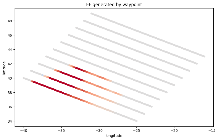
[20]:
# Visualize the "ef" of each flight
ax = plt.axes()
for fl in output_flights:
    fl.dataframe.plot.scatter(
        x="longitude",
        y="latitude",
        c="ef",
        cmap="coolwarm",
        vmin=-3e13,
        vmax=3e13,
        title="EF generated by waypoint",
        ax=ax,
        colorbar=False,
    )
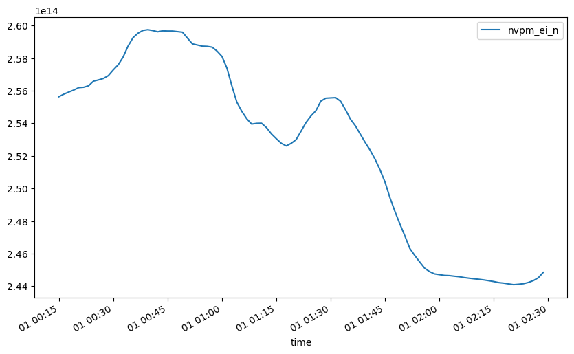
Use the Poll-Schumann aircraft performance model
First create a Flight that does not have emissions data associated:
[21]:
from pycontrails.models.ps_model import PSFlight
[22]:
# demo synthetic flight
flight_attrs = {
    "flight_id": "test-ps-model",
    "aircraft_type": "E195",
}

# Example flight
df = pd.DataFrame()
df["longitude"] = np.linspace(-40, -55, 100)
df["latitude"] = np.linspace(38, 45, 100)
df["altitude"] = np.linspace(10900, 10900, 100)
df["time"] = pd.date_range("2022-03-01T00:15:00", "2022-03-01T02:30:00", periods=100)
fl = Flight(data=df, attrs=flight_attrs)
[23]:
cocip = Cocip(
    met=met,
    rad=rad,
    humidity_scaling=ConstantHumidityScaling(rhi_adj=0.99),
    aircraft_performance=PSFlight(),
)

output_flight = cocip.eval(source=fl)
[24]:
output_flight.dataframe.plot(x="time", y="nvpm_ei_n");
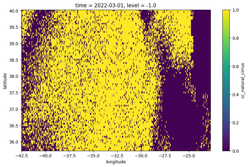
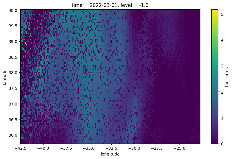
Output contrail cirrus optical depth
Note this is only a preliminary implementation and will be changed in the future
The example below uses the contrail cirrus output from 1 flight, but the df_contrails input can include contrail cirrus from multiple flights.
To run multiple flights, concatenate Cocip.contrail outputs from multiple flights and feed in to grid_cirrus.<> methods as df_contrails. Unique flight_id column will have to be added to the Cocip.contrail output before concatenation.
[25]:
from pycontrails.models.cocip import natural_cirrus_properties_to_hi_res_grid
[26]:
# demo synthetic flight
flight_attrs = {
    "flight_id": "test",
    "true_airspeed": 226.099920796651,  # true airspeed, m/s
    "thrust": 0.22,  # thrust_setting
    "nvpm_ei_n": 1.897462e15,
    "aircraft_type": "E190",
    "wingspan": 48,
    "n_engine": 2,
}

# Example flight
df = pd.DataFrame()
df["longitude"] = np.linspace(-40, -55, 100)
df["latitude"] = np.linspace(38, 45, 100)
df["altitude"] = np.linspace(10900, 10900, 100)
df["engine_efficiency"] = np.linspace(0.34, 0.35, 100)  # ope
df["fuel_flow"] = np.linspace(2.1, 2.4, 100)  # kg/s
df["aircraft_mass"] = np.linspace(154445, 154345, 100)  # kg
df["time"] = pd.date_range("2022-03-01T00:15:00", "2022-03-01T02:30:00", periods=100)
fl = Flight(data=df, attrs=flight_attrs)
[27]:
# run model
cocip = Cocip(
    met=met,
    rad=rad,
    process_emissions=False,
    humidity_scaling=ConstantHumidityScaling(rhi_adj=0.99),
)
output_flight = cocip.eval(source=fl)
[28]:
# get dataframe of contrail waypoints
df_contrails = cocip.contrail
df_contrails["flight_id"] = cocip.source.attrs["flight_id"]
[29]:
w = df_contrails["longitude"].min()
e = df_contrails["longitude"].max()
s = df_contrails["latitude"].min()
n = df_contrails["latitude"].max()
bbox = (w, s, e, n)

met_bbox = MetDataset(met.data.isel(time=[0])).downselect(bbox)
[30]:
ds_cirrus = natural_cirrus_properties_to_hi_res_grid(met_bbox)
/Users/marcshapiro/computing/contrailcirrus/pycontrails/pycontrails/core/met.py:802: UserWarning: Overwriting data in keys `['tau_cirrus']`. Use `.update(...)` to suppress warning.
  warnings.warn(
[31]:
ds_cirrus["cc_natural_cirrus"].data.squeeze().plot(x="longitude", y="latitude");
[32]:
ds_cirrus["tau_cirrus"].data.squeeze().plot(x="longitude", y="latitude");
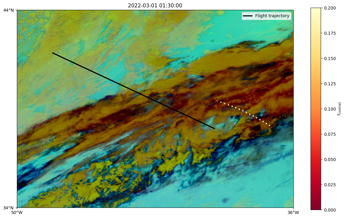
Compare CoCiP outputs with GOES imagery
Requires the pycontrails[goes] optional dependencies.
[33]:
from pycontrails.models.cocip import compare_cocip_with_goes
[34]:
# demo synthetic flight
flight_attrs = {
    "flight_id": "test",
    "true_airspeed": 226.099920796651,  # true airspeed, m/s
    "thrust": 0.22,  # thrust_setting
    "nvpm_ei_n": 1.897462e15,
    "aircraft_type": "E190",
    "wingspan": 48,
    "n_engine": 2,
}

# Example flight
df = pd.DataFrame()
df["longitude"] = np.linspace(-40, -55, 100)
df["latitude"] = np.linspace(38, 45, 100)
df["altitude"] = np.linspace(10900, 10900, 100)
df["engine_efficiency"] = np.linspace(0.34, 0.35, 100)  # ope
df["fuel_flow"] = np.linspace(2.1, 2.4, 100)  # kg/s
df["aircraft_mass"] = np.linspace(154445, 154345, 100)  # kg
df["time"] = pd.date_range("2022-03-01T00:15:00", "2022-03-01T02:30:00", periods=100)
fl = Flight(data=df, attrs=flight_attrs)
[35]:
# run model
cocip = Cocip(
    met=met,
    rad=rad,
    process_emissions=False,
    humidity_scaling=ConstantHumidityScaling(rhi_adj=0.99),
)
output_flight = cocip.eval(source=fl)
[38]:
compare_cocip_with_goes(
    time=pd.Timestamp("2022-03-01T01:30:00"),
    flight=output_flight,
    contrail=cocip.contrail,
    spatial_bbox=(-50, 34, -36, 44),
)