Find and retrieve Landsat imagery¶

This notebook demonstrates how to: - intersect Landsat scenes with a flight track using BigQuery - retrieve and visualized Landsat scenes

This notebook relies on optional dependencies in the sat group (pip install pycontrails[sat]).

[1]:

import matplotlib.pyplot as plt
import numpy as np
import pandas as pd
import pyproj
from matplotlib import dates

from pycontrails.core import Flight
from pycontrails.datalib import landsat

Intersect Landsat scenes with IAGOS flight¶

Intersecting Landsat scenes with flight tracks requires a Google Cloud account and project with access to the BigQuery API. Users without BigQuery API access can skip this section.

[2]:

df = pd.read_csv("data/iagos-flight-landsat.csv")
df["time"] = df["time"].apply(lambda t: pd.Timestamp(t))

[3]:

flight = Flight(data=df).resample_and_fill("1min")

[4]:

scenes = landsat.intersect(flight)
scenes

[4]:

	base_url	sensing_time
0	gs://gcp-public-data-landsat/LC08/01/124/048/L...	2019-01-12 03:05:55.144026+00:00
1	gs://gcp-public-data-landsat/LC08/01/124/049/L...	2019-01-12 03:06:19.047773+00:00

Retrieve and visualize Landsat scene¶

This section retrieves Landsat imagery from a Google Cloud public dataset. Retrieval uses anonymous access, so this section of the notebook can be run by users without a Google Cloud account.

The base_url used here corresponds to the first scene found in the previous section. In the second scene, the flight is in a region with missing imagery. Both base_url and sensing_time are hard-coded so this section can be run independently of the previous section.

[5]:

base_url = "gs://gcp-public-data-landsat/LC08/01/124/048/LC08_L1TP_124048_20190112_20190131_01_T1"
sensing_time = pd.Timestamp("2019-01-12 03:05:55.144026+00:00")

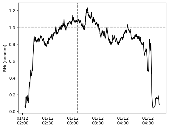
The IAGOS flight is in an ISSR at the time of imagery acquisition:

[6]:

plt.plot(df["time"], df["rhi"], "k-")
plt.ylabel("RHi (nondim)")
plt.gca().xaxis.set_major_formatter(dates.DateFormatter("%m/%d\n%H:%M"))
plt.gca().axhline(y=1, color="gray", ls="--")
plt.gca().axvline(x=sensing_time, color="gray", ls="--");

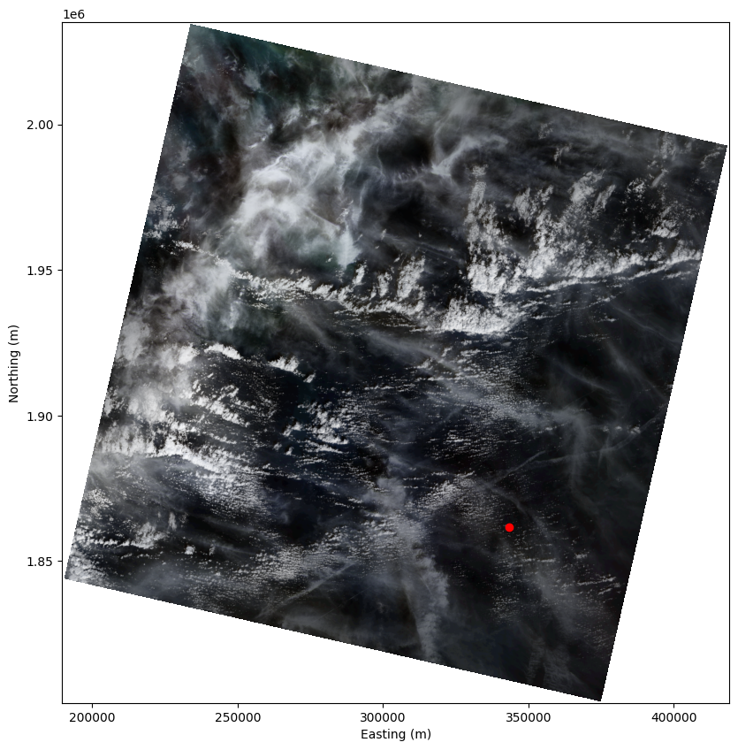
True-color image¶

We first download bands 2, 3, and 4. These are used to create a true-color image.

Note that handler.get transfers satellite imagery from a Google Cloud bucket to your machine. This may take a while if you are running this notebook locally rather than on a Google Cloud VM.

[7]:

handler = landsat.Landsat(base_url, bands=["B2", "B3", "B4"])
ds = handler.get()
ds

We then generate and plot the true-color image.

[8]:

rgb, crs, extent = landsat.extract_landsat_visualization(ds, color_scheme="true")

[9]:

# crs artifact can be used to project flight latitude and longitude into image coordinates
proj = pyproj.Transformer.from_crs(crs.geodetic_crs, crs)
flight_lon = np.interp(
    sensing_time.timestamp(),
    df["time"].apply(lambda t: pd.Timestamp(t).timestamp()),
    df["longitude"],
)
flight_lat = np.interp(
    sensing_time.timestamp(),
    df["time"].apply(lambda t: pd.Timestamp(t).timestamp()),
    df["latitude"],
)
flight_x, flight_y = proj.transform(flight_lat, flight_lon)

[10]:

plt.figure(figsize=(10, 10))
plt.imshow(rgb, extent=extent)
plt.plot(flight_x, flight_y, "ro")
plt.xlabel("Easting (m)")
plt.ylabel("Northing (m)");

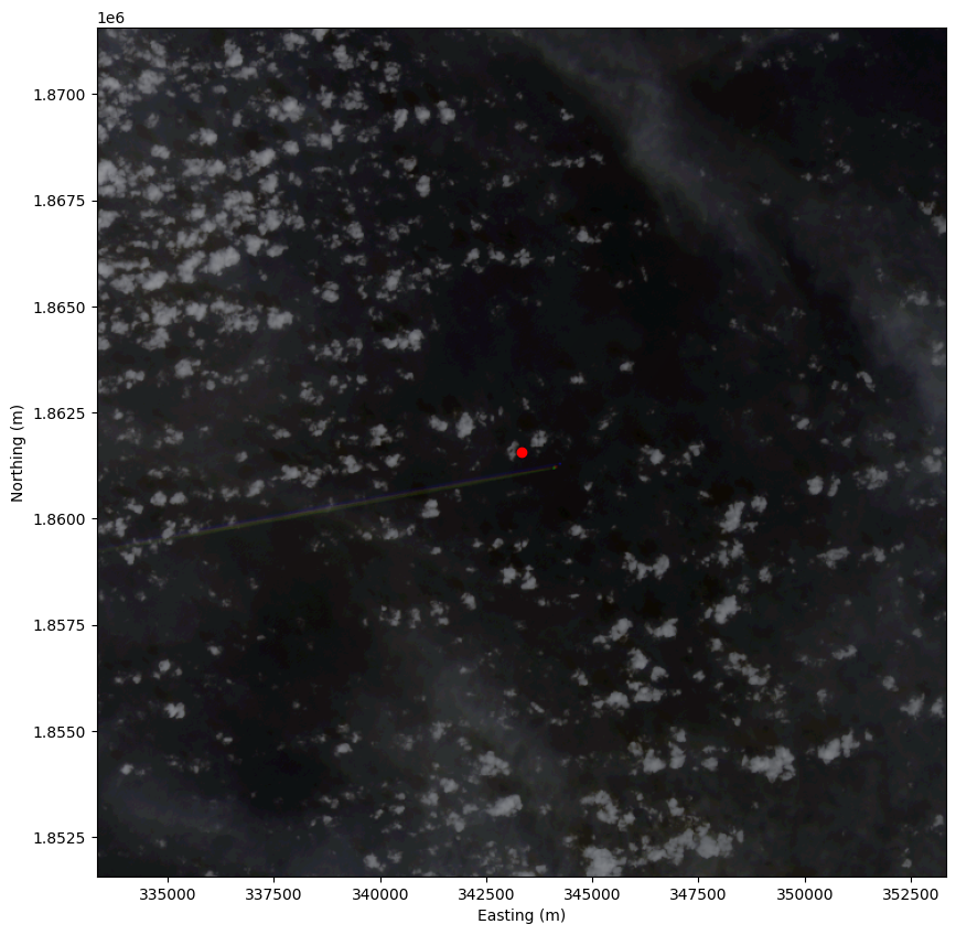
If we zoom in, we can see the aircraft and contrail! The aircraft is offset slightly from its projected position because Landsat imagery is geolocated at the surface.

[11]:

plt.figure(figsize=(10, 10))
plt.imshow(rgb, extent=extent)
plt.plot(flight_x, flight_y, "ro")
plt.xlim([flight_x - 10e3, flight_x + 10e3])
plt.ylim([flight_y - 10e3, flight_y + 10e3])
plt.xlabel("Easting (m)")
plt.ylabel("Northing (m)");

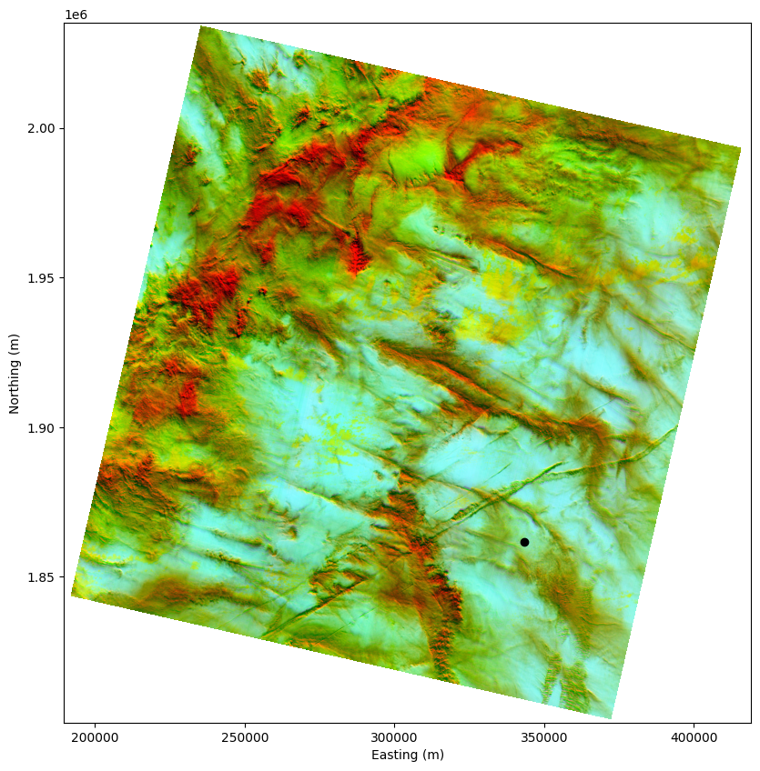
False-color thermal image¶

Finally, we download bands 9, 10, and 11 and use them to create a false-color image using a color scheme designed for contrail detection by Google Research.

[12]:

handler = landsat.Landsat(base_url, bands=["B9", "B10", "B11"])
ds = handler.get()

[13]:

rgb, crs, extent = landsat.extract_landsat_visualization(ds, color_scheme="google_contrails")

[14]:

proj = pyproj.Transformer.from_crs(crs.geodetic_crs, crs)
flight_x, flight_y = proj.transform(flight_lat, flight_lon)

[15]:

plt.figure(figsize=(10, 10))
plt.imshow(rgb, extent=extent)
plt.plot(flight_x, flight_y, "ko")
plt.xlabel("Easting (m)")
plt.ylabel("Northing (m)");